NB the Jupyter notebook includes interactive widgets that are very useful for building an understanding of these models.
Departmental punctuality
Imagine that your university hires a new president. On her first week, she schedules a meeting with professors from three departments, { D = \{ \text{G}, ~ \text{E}, ~ \text{M} \} }. The professor from the Department of Government ({ d{=}\text{G} }) shows up 1 minute late, the professor from the Department of English ({ d{=}\text{E} }) shows up 15 minutes before the scheduled meeting time, and the professor from the Department of Math ({ d{=}\text{M} }) shows up 30 minutes late. From this single meeting the new president updates her beliefs about when professors will show up to scheduled meetings.
But how should the president update her beliefs? It could be that departments have different relationships with punctuality and it would be useful to expect professors from the Math department to show up later than professors from the English department. It could also be the case that there is not meaningful between-department variance and she should just learn about the greater population of professors at the university.
A model that infers information about the population without differentiating subpopulations is doing “complete pooling”, meaning that all of the variance in the data is treated as being generated by the same distribution. I.e. the data is pooled together and treated as iid observations drawn from a single distribution.
If the president thinks of each department independently, what she learns about the punctuality of professors from one department will not change her beliefs about professors from other departments. In this case, there would be “no pooling” of information across departments. The president’s observations of the three professors would have no bearing on her belief about what to expect of a professor from a fourth department (e.g. Psychology).
“Partial pooling” models represent uncertainty at multiple levels of abstraction. Based on her observations from this meeting, the president will update her beliefs about these departments as well as the greater population. In other words, what she observes about the Math department might strongly update her beliefs about that department, moderately update her beliefs about the broader population, and that in turn could weakly update her beliefs about the English department.
Complete pooling
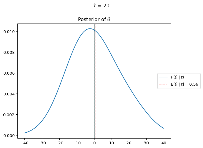
Let’s build a complete pooling model of the president’s belief about the punctuality of professors. The data observed by the president are { t = \langle t_G, t_E, t_M \rangle = \langle 1, -15, 30 \rangle }. We’ll model the president’s belief about the greater population of professors as a normal distribution centered at \theta with standard deviation \dot\sigma. Prior to meeting with anyone, the president thinks that professors will, on average, show up on time, but that some will show up early and some late. We can encode this prior belief as a normal distribution centered at zero, with some standard deviation, let’s say 20. I.e. the prior for \theta is:
If she observes that professors tend to be late, then her posterior estimate of \theta will have an expected value greater than zero (i.e. { \operatorname{E}[\theta \mid t] > 0 }), and if she ends up expecting professors to be early, then { \operatorname{E}[\theta \mid t] < 0 }.
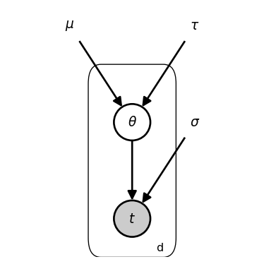
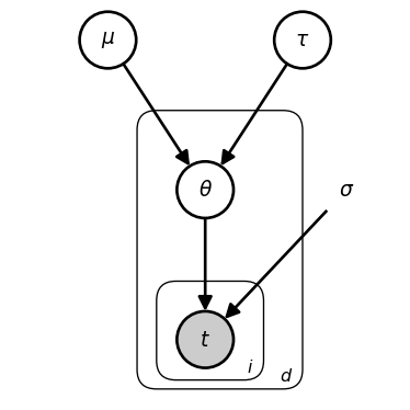
In this tutorial I’ll use a dot above to indicate that a variable is fixed, not inferred. (N.B. the dot is not standard notation, just what I’m using here.) In the graphical schematic, fixed parameters are depicted as bare symbols rather than nodes. Note that “fixed” means the values are not updated during inference (but you can, of course, manually tune these values or learn suitable values by minimizing some loss function in conjunction with a model fitting algorithm).
Since the model infers the distribution of \theta, the graphical schematic depicts it as an open node (i.e. a latent random variable). The data in this model are t.
We specify the likelihood as,
t_d ~\sim~ \mathcal{N}(\theta, ~ \dot\sigma{=}15)
I.e., for whatever the true value of \theta is for the population of professors, the president thinks that when professors actually show up will follow a normal distribution, centered on the true value of \theta, with standard deviation 15.
%reset -fimport jaximport jax.numpy as jnpfrom memo import memofrom enum import IntEnumfrom jax.scipy.stats.norm import pdf as normpdffrom jax.scipy.stats.cauchy import pdf as cauchypdffrom matplotlib import pyplot as pltnormpdfjit = jax.jit(normpdf)class Department(IntEnum): GOVERNMENT =0 ENGLISH =1 MATH =2t = jnp.array([1, -15, 30])sigma =15Theta = jnp.linspace(-40, 40, 200)@jax.jitdef professor_arrival_likelihood(d, theta):### likelihood of a professor from department d ### showing up t_d minutes early/late, ### under the hypothesis given by theta and sigma.return normpdf(t[d], loc=theta, scale=sigma)@memodef complete_pooling[ _theta: Theta,](mu=0, tau=1): president: knows(_theta) president: thinks[ department: chooses(theta in Theta, wpp=normpdfjit(theta, mu, tau)) ] president: observes_event( wpp=professor_arrival_likelihood({Department.GOVERNMENT}, department.theta)) president: observes_event( wpp=professor_arrival_likelihood({Department.ENGLISH}, department.theta)) president: observes_event( wpp=professor_arrival_likelihood({Department.MATH}, department.theta))return president[Pr[department.theta == _theta]]mu_ =0tau_ =20res = complete_pooling(mu=mu_, tau=tau_)### check the size and sum of the output# res.shape# res.sum()fig, ax = plt.subplots()ax.axvline(0, color="black", linestyle="-")theta_posterior = restheta_expectation = jnp.dot(Theta, theta_posterior)ax.plot(Theta, theta_posterior, label=r"$P(\theta \mid t)$")ax.axvline( theta_expectation, color='red', linestyle='--', label=(r"$\operatorname{E}"+rf"[\theta \mid t]={theta_expectation:6.2f}$"))_ = ax.set_title(r"Posterior of $\theta$")_ = ax.legend(bbox_to_anchor=(0.9, 0.5), loc='center left')_ = plt.suptitle(fr"$\dot\tau$ = {tau_}", y=1)plt.tight_layout()plt.show()
Try changing the data to t = jnp.array([-20, -10, 30]). Notice how changing the data for one group updates the expectation of the population.
No pooling
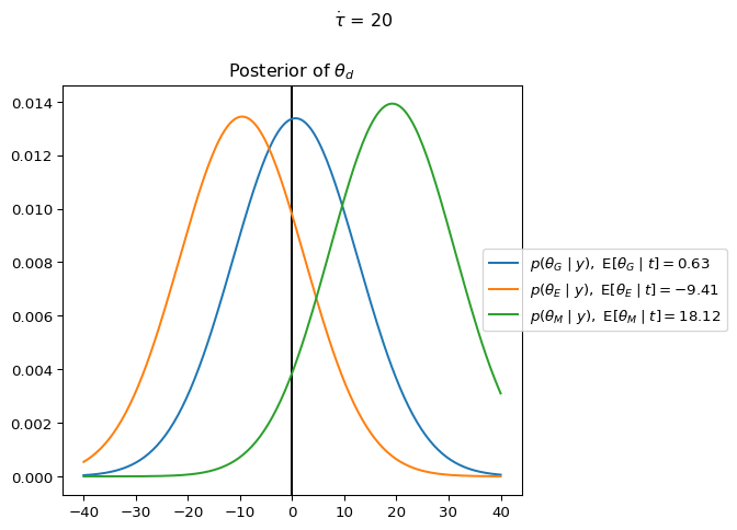
In contrast to complete pooling, which assumes all observations are generated by a shared population-level distribution parameterized by \theta, the no pooling model treats each department as having its own independent parameter \theta_d. The key change is that instead of having a single \theta drawn from the prior distribution, we now have three independent parameters \theta_G, \theta_E, and \theta_M. The practical meaning of this change is significant:
In complete pooling, an observation of the Math professor being late would shift our expectations for all departments. In no pooling, learning that the Math professor is late only updates our beliefs about the Math department. Each department’s parameter is estimated using only data from that department.
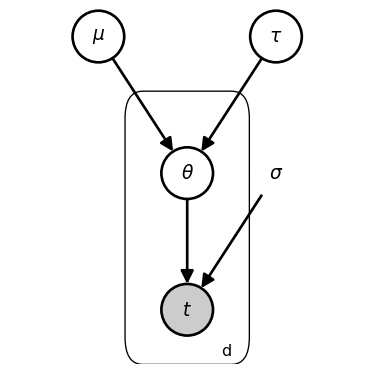
The key change in our model specification is that we have replaced the single \theta with three parameters, \theta_d.
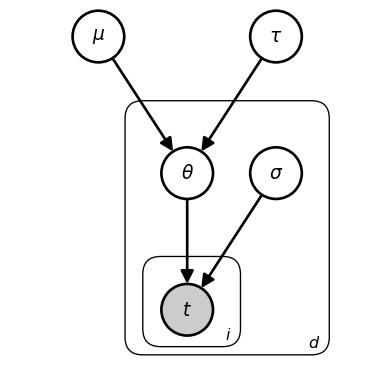
The plate (rectangular box) with label d indicates that everything inside is repeated for each department d \in \mathcal{D}. Variables inside the plate have a unique value for each department. Variables outside the plate are shared across all departments.
To change the complete_pooling model to the no_pooling model we make a simple change, adding the conditional statement
president: observes [department.d] is _d
and the query variable _d in the definition, [_d: Department, ...].
%reset -fimport jaximport jax.numpy as jnpfrom memo import memofrom enum import IntEnumfrom jax.scipy.stats.norm import pdf as normpdffrom jax.scipy.stats.cauchy import pdf as cauchypdffrom matplotlib import pyplot as pltnormpdfjit = jax.jit(normpdf)class Department(IntEnum): GOVERNMENT =0 ENGLISH =1 MATH =2t = jnp.array([1, -15, 30])sigma =15Theta = jnp.linspace(-40, 40, 200)@jax.jitdef professor_arrival_likelihood(d, theta):### likelihood of a professor from department d ### showing up t_d minutes early/late, ### under the hypothesis given by theta and sigma.return normpdf(t[d], loc=theta, scale=sigma)@memodef no_pooling[ _d: Department, _theta: Theta,](mu=0, tau=1): president: knows(_theta) president: thinks[ department: chooses(d in Department, wpp=1), department: chooses(theta in Theta, wpp=normpdfjit(theta, mu, tau)) ] president: observes [department.d] is _d ### new conditional statement president: observes_event( wpp=professor_arrival_likelihood(department.d, department.theta))return president[Pr[department.theta == _theta]]mu_ =0tau_ =20res = no_pooling(mu=mu_, tau=tau_)### check the size and sum of the output# res.shape# res.sum()# res[0].sum()# res[1].sum()# res[2].sum()fig, ax = plt.subplots()ax.axvline(0, color="black", linestyle="-")for d in Department: department_name = d.name department_abbrev = department_name[0] theta_posterior = res[d] theta_expectation = jnp.dot(Theta, theta_posterior) ax.plot( Theta, theta_posterior, label=(rf"$p(\theta_{department_abbrev}\mid t),~ "+r"\operatorname{E}"+rf"[\theta_{department_abbrev}\mid t]={theta_expectation:6.2f}$") )_ = ax.set_title(r"Posterior of $\theta_d$")_ = ax.legend(bbox_to_anchor=(0.9, 0.5), loc='center left')_ = plt.suptitle(fr"$\dot\tau$ = {tau_}", y=1)plt.tight_layout()plt.show()
Try changing the data to t = jnp.array([-20, -15, 30]). Notice how changing the data for one group does not affect the expectation of the posterior of the other groups.
Previously, the complete_pooling model returned an array of shape (200,) with 200 being the size of the sample space of Theta. With the addition of the conditional statement, what array shape does no_pooling return? Make sure you understand the shape change, what each dimension reflects, and why the values sum in the ways that they do.
The key theoretical distinction is that in no pooling, we’re asserting that the timing behavior of professors in different departments is independent of the behavior of professors from other departments (i.e. when professors from one department show up for meetings carries no information about when professors from a different department will show up). This is an unrealistically strong assumption.
The no_pooling and complete_pooling models highlight an important practical tradeoff: no pooling can better capture differences between departments but may suffer from high variance in its estimates due to small sample sizes within each department. Complete pooling has lower variance but may miss important systematic differences between departments.
Partial pooling
In partial pooling, every observation updates beliefs across multiple levels of abstraction. The critical insight is that while departments may differ in their typical timing behavior, the departments are not statistically independent. They are influenced by common causes. To model the president’s reasoning about these multiple levels of uncertainty, we modify the no_pooling model by adding priors over \mu and \tau.
Rather than being fixed values, \mu and \tau become latent parameters to be jointly inferred alongside \theta_d.
The higher-level latent parameters \mu and \tau characterize a “population-level” distribution from which department-specific \theta_d values are generated.
The key change to the model is that rather than { \theta_d ~\sim~ \mathcal{N}\left( \dot{\mu}{=}0, ~ \dot{\tau}{=}20 \right) }, we have { \theta_d ~\sim~ \mathcal{N}\left(\mu, ~ \tau \right) } and specify hyperpriors on these new latent parameters: { \mu ~\sim~ \mathcal{N}(0, ~ \dot\sigma_{\mu}) } and { \tau ~\sim~ \text{HalfCauchy}(\dot\sigma_{\tau}) }.
Note that there are new fixed parameters: mu_scale ({ \dot\sigma_\mu}) and tau_scale ({ \dot\sigma_\tau }), but I am omitting there from the graphical schematic for the sake of visual simplicity.
%reset -fimport jaximport jax.numpy as jnpfrom memo import memofrom enum import IntEnumfrom jax.scipy.stats.norm import pdf as normpdffrom jax.scipy.stats.cauchy import pdf as cauchypdffrom matplotlib import pyplot as pltnormpdfjit = jax.jit(normpdf)class Department(IntEnum): GOVERNMENT =0 ENGLISH =1 MATH =2t = jnp.array([1, -15, 30])sigma =15Mu = jnp.linspace(-25, 25, 100) ### sample space for new hyperpriorTau = jnp.linspace(1, 30, 100) ### sample space for new hyperpriorTheta = jnp.linspace(-40, 40, 200)### PDF for new hyperprior@jax.jitdef half_cauchy(x, scale=1.0):return2* cauchypdf(x, 0, scale)@jax.jitdef professor_arrival_likelihood(d, theta):### likelihood of a professor from department d ### showing up t_d minutes early/late, ### under the hypothesis given by theta and sigma.return normpdf(t[d], loc=theta, scale=sigma)@memodef department_model[_mu: Mu, _tau: Tau](d): department: knows(_mu, _tau) department: chooses(theta in Theta, wpp=normpdfjit(theta, _mu, _tau))return E[ department[professor_arrival_likelihood(d, theta)] ]@memodef partial_pooling[_mu: Mu, _tau: Tau](mu_scale=5, tau_scale=5): president: knows(_mu, _tau) president: thinks[ population: chooses(mu in Mu, wpp=normpdfjit(mu, 0, mu_scale)), population: chooses(tau in Tau, wpp=half_cauchy(tau, tau_scale)), ] president: observes_event( wpp=department_model[population.mu, population.tau]({Department.GOVERNMENT})) president: observes_event( wpp=department_model[population.mu, population.tau]({Department.ENGLISH})) president: observes_event( wpp=department_model[population.mu, population.tau]({Department.MATH}))return president[Pr[population.mu == _mu, population.tau == _tau]]
Let’s think about what each variable represents.
The likelihood model professor_arrival_likelihood gives the probability that a professor from department d shows up t_d minutes early/late, under a given \theta_d and \sigma:
We can write the likelihood as { P(t_d \mid \theta_d, ~ \mu, ~\tau ~;~ \sigma) }. The marginal posterior { P(\theta_d \mid t) } will thus represent the president’s belief about the true value of \theta_d for a given department d.
@memodef department_model_theta[_theta: Theta](d, mu_scale, tau_scale): obs: thinks[ department: chooses(mu in Mu, tau in Tau, wpp=partial_pooling[mu, tau](mu_scale, tau_scale)), department: chooses(theta in Theta, wpp=normpdfjit(theta, mu, tau)) ] obs: observes_event(wpp=professor_arrival_likelihood(d, department.theta)) obs: knows(_theta)return obs[Pr[department.theta == _theta]]
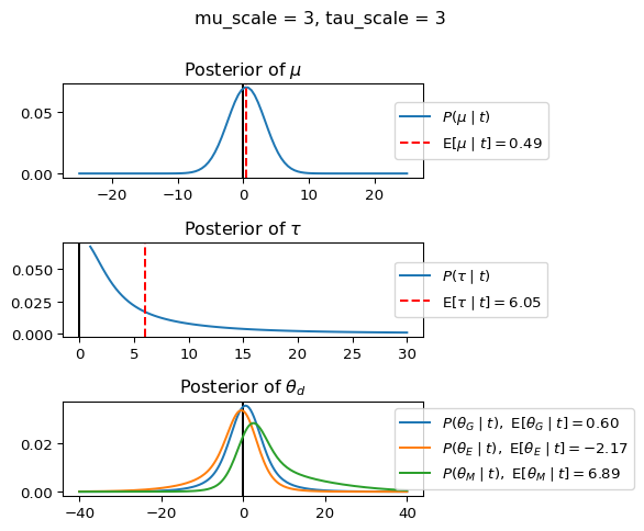
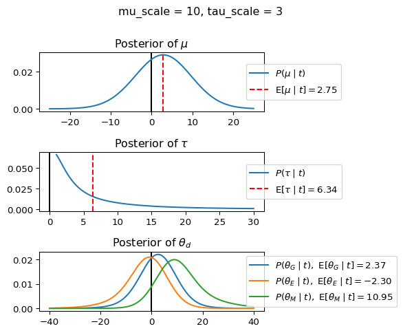
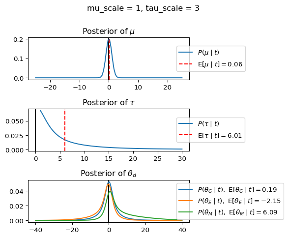
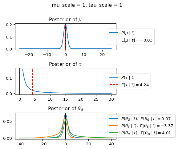
When mu_scale is small (e.g. { \dot\sigma_{\mu}{=}1 }) the location of the distribution over \theta_d will be centered near zero. When mu_scale is large (e.g. { \dot\sigma_{\mu}{=}10 }), the center of { \mathcal{N}(\mu, ~ \tau) } can move to new locations with greater freedom. This results in a more flexible population-level mean, allowing the model to adapt to data that suggests professors generally arrive early or late across all departments. With a large mu_scale, the model places less prior constraint on where the overall population mean should be, letting the data have more influence on determining this parameter.
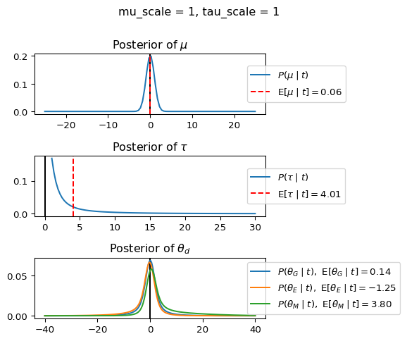
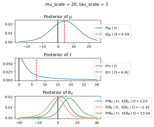
When tau_scale is small (e.g. { \dot\sigma_{\tau}{=}1 }), the distribution { \theta_d ~\sim~ \mathcal{N}(\mu, ~ \tau) } will be narrow, which will result in strong shrinkage of department-specific means toward the overall population mean. This effectively reduces the differences between departments, making the model behave more like the complete pooling model. The practical interpretation is that the model assumes departments are relatively homogeneous in their timing behavior.
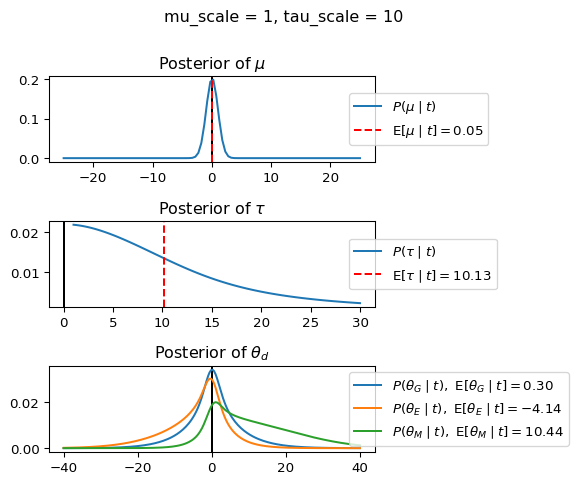
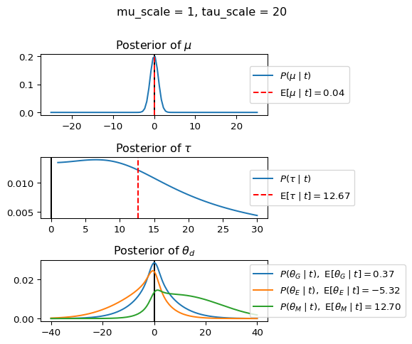
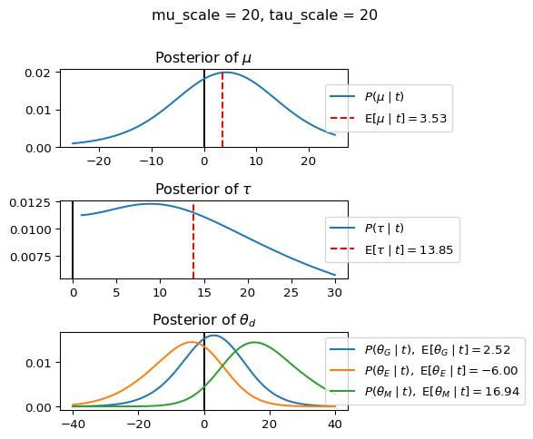
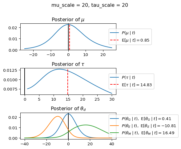
When tau_scale is large (e.g. { \dot\sigma_{\tau}{=}20 }), the { \theta_d } can diverge more freely from the population mean, resulting in weaker shrinkage effects. Department-specific estimates will be closer to their empirical means and less influenced by data from other departments. This allows the model to capture more heterogeneity between departments, making it behave more like the no pooling model while still maintaining some information sharing.
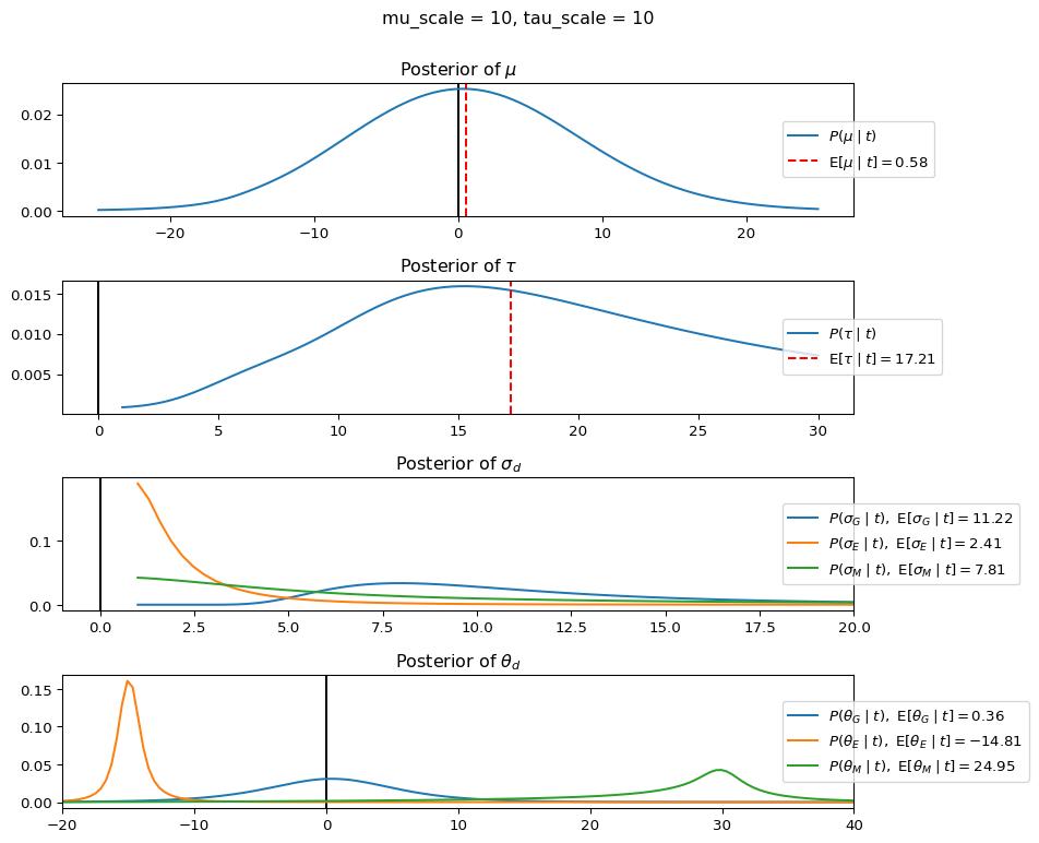
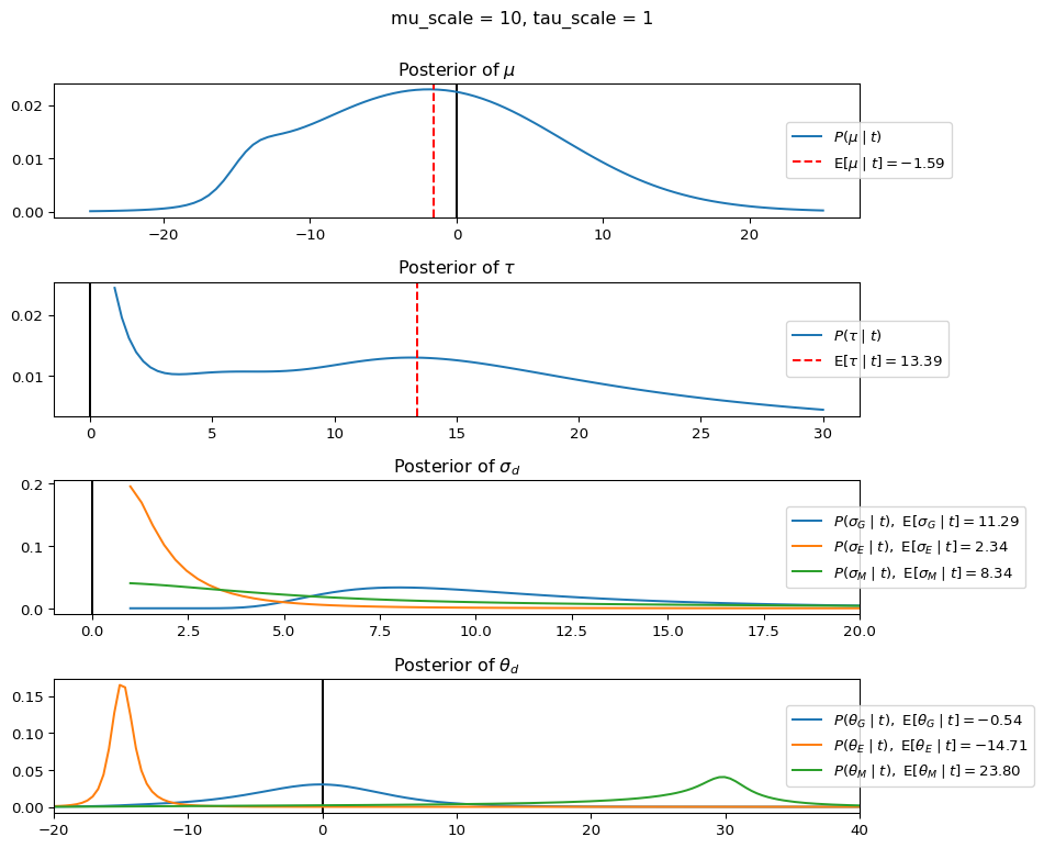
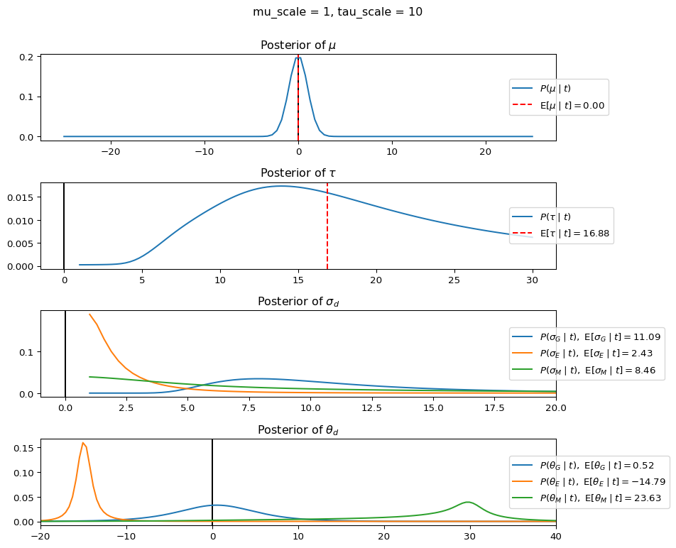
In this way, a large { \dot\sigma_{\mu} } and small { \dot\sigma_{\tau} } would create a model that assumes departments are relatively homogeneous (due to small \tau) but is very flexible about where the overall population mean might be (due to large \mu scale). This combination would result in strong shrinkage of department-specific estimates toward a population mean that is itself quite adaptable to the data. Conversely, a small { \dot\sigma_{\mu} } and large { \dot\sigma_{\tau} } would create a model with a strong prior belief the population mean is near zero, but allows substantial variation between departments.
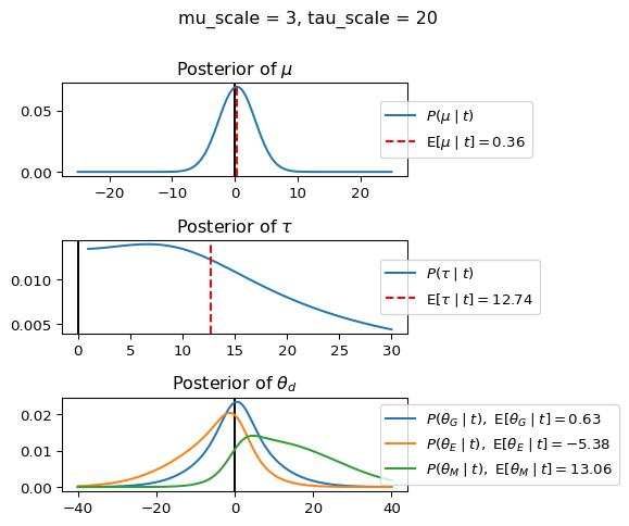
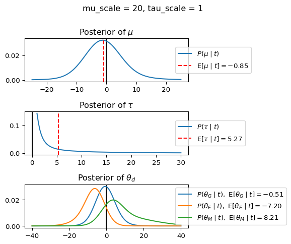
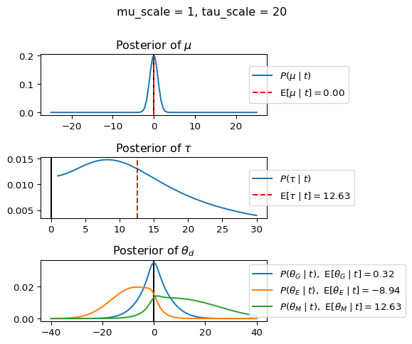
What if the president instead had a large meeting with 7 professors and the departments were not equally represented? How would she update her beliefs given unequal observations? Let’s say that she invited 3 professors from the Department of Government, 3 from the Department of English, and 1 from the Department of Math. We can explore how modulating the higher-level hyperpriors changes her posterior inference about each department.
When tau_scale is small (e.g. { \dot\sigma_{\tau}{=}1 }), the distribution { \theta_d ~\sim~ \mathcal{N}(\mu, ~ \tau) } will be narrow, which will pressure the individual { \theta_d } to be similar to each other. When tau_scale is large (e.g. { \dot\sigma_{\tau}{=}20 }), the { \theta_d } can diverge more freely resulting in values quite different from each other. Think about how this will interact with the number of observations and the values of those observations.
When mu_scale is small (e.g. { \dot\sigma_{\mu}{=}1 }) the location of the distribution over \theta_d will be be centered near zero. When mu_scale is large (e.g. { \dot\sigma_{\mu}{=}20 }), the center of { \mathcal{N}(\mu, ~ \tau) } can move to new locations.
In this way, a large { \dot\sigma_{\mu} } and small { \dot\sigma_{\tau} } would allow { \mathcal{N}(\mu, ~ \tau) } to move to easily move to a new location that accommodates the broader tendencies of departments and professors, but would constrain the dispersion between departments. Notice how increasing mu_scale allows the posterior { P(\mu \mid t) } to move away from zero towards the mean of the combined data, whereas decreasing mu_scale pulls the expectation { \operatorname{E}[\mu \mid t] } towards zero. Also notice how this effect is stronger when tau_scale is small.
Pay close attention to the interaction between mu_scale, tau_scale, and the observations for each department (including the expectation and variance of the observations of each department).
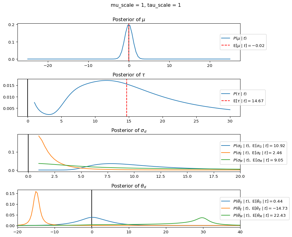
Multiple observations with missing data and learned variance
%reset -fimport jaximport jax.numpy as jnpfrom memo import memofrom enum import IntEnumfrom jax.scipy.stats.norm import pdf as normpdffrom jax.scipy.stats.norm import logpdf as normlogpdffrom jax.scipy.stats.cauchy import pdf as cauchypdffrom matplotlib import pyplot as pltnormpdfjit = jax.jit(normpdf)class Department(IntEnum): GOVERNMENT =0 ENGLISH =1 MATH =2t = jnp.array([ [-10, 1, 11], [-16, -15, -14], [30, jnp.nan, jnp.nan],])Mu = jnp.linspace(-25, 25, 100)Tau = jnp.linspace(1, 30, 100)Theta = jnp.linspace(-40, 40, 200)Sigma = jnp.linspace(1, 30, 100) ###NEW@jax.jitdef half_cauchy(x, scale=1.0):return2* cauchypdf(x, 0, scale)@jax.jitdef professor_arrival_likelihood(d, theta, sigma): ###NEW### likelihood of a professor from department d ### showing up t_d minutes early/late, ### under the hypothesis given by theta and sigma.return jnp.exp(jnp.nansum(normlogpdf(t[d], theta, sigma)))@memo(cache=True)def department_model[_mu: Mu, _tau: Tau](d): department: knows(_mu, _tau) department: chooses(theta in Theta, wpp=normpdfjit(theta, _mu, _tau)) department: chooses(sigma in Sigma, wpp=half_cauchy(sigma, 5)) ###NEWreturn E[ department[professor_arrival_likelihood(d, theta, sigma)] ] ###NEW@memo(cache=True)def partial_pooling[_mu: Mu, _tau: Tau](mu_scale=5, tau_scale=5): president: knows(_mu, _tau) president: thinks[ population: chooses(mu in Mu, wpp=normpdfjit(mu, 0, mu_scale)), population: chooses(tau in Tau, wpp=half_cauchy(tau, tau_scale)), ] president: observes_event(wpp=department_model[population.mu, population.tau]({Department.GOVERNMENT})) president: observes_event(wpp=department_model[population.mu, population.tau]({Department.ENGLISH})) president: observes_event(wpp=department_model[population.mu, population.tau]({Department.MATH}))return president[Pr[population.mu == _mu, population.tau == _tau]]@memo(cache=True)def department_model_theta[_theta: Theta](d, mu_scale, tau_scale): obs: thinks[ department: chooses(mu in Mu, tau in Tau, wpp=partial_pooling[mu, tau](mu_scale, tau_scale)), department: chooses(theta in Theta, wpp=normpdfjit(theta, mu, tau)), department: chooses(sigma in Sigma, wpp=half_cauchy(sigma, 5)), ###NEW ] obs: observes_event(wpp=professor_arrival_likelihood(d, department.theta, department.sigma)) ###NEW obs: knows(_theta)return obs[Pr[department.theta == _theta]]@memo(cache=True)def department_model_sigma[_sigma: Sigma](d, mu_scale, tau_scale): ###NEW obs: thinks[ department: chooses(mu in Mu, tau in Tau, wpp=partial_pooling[mu, tau](mu_scale, tau_scale)), department: chooses(theta in Theta, wpp=normpdfjit(theta, mu, tau)), department: chooses(sigma in Sigma, wpp=half_cauchy(sigma, 5)), ] obs: observes_event(wpp=professor_arrival_likelihood(d, department.theta, department.sigma)) obs: knows(_sigma)return obs[Pr[department.sigma == _sigma]]
Caching function
# Cache for precomputed resultscache = {}def compute_distributions(mu_scale, tau_scale, verbose=False):"""Retrieve from cache or compute the JAX-based distributions.""" key = (mu_scale, tau_scale)if key in cache:return cache[key] # Use cached resultsif verbose:print(f"{mu_scale=}, {tau_scale=}")# Cache results cache[key] = ( partial_pooling(mu_scale=mu_scale, tau_scale=tau_scale).sum(axis=1), partial_pooling(mu_scale=mu_scale, tau_scale=tau_scale).sum(axis=0), {d: department_model_sigma(d, mu_scale, tau_scale) for d in Department}, {d: department_model_theta(d, mu_scale, tau_scale) for d in Department}, )return cache[key]
Gelman, Andrew, Carlin, John B., Stern, Hal S., Dunson, David B., Vehtari, Aki, & Rubin, Donald B. (2014). Bayesian data analysis (Third edition). CRC Press, Taylor & Francis Group.
Kruschke, John K. (2015). Doing Bayesian data analysis: A tutorial introduction with R, JAGS, and Stan (Edition 2). Elsevier, Academic Press.
McElreath, Richard. (2016). Statistical rethinking: A Bayesian course with examples in R and Stan. CRC Press/Taylor & Francis Group.