Bayes’ rule

Imagine you have a bag with 10 coins in it. Of these coins, 9 are fair and 1 is biased with {P(\text{H}) = 0.9}. The biased coin is painted red.

You pull a coin from the bag, look at it, and flip it three times. You record the sequence and whether it was the biased coin or a fair coin. You then put the coin back in the bag. You repeat this thousands of times until you have an estimate of the probability of every sequence, both for the biased coin and for a fair coin.

You now pass the bag to a friend and close your eyes. Your friend draws a coin, flips it three times, and tells you all three flips came up \text{H}. What’s the probability that your friend flipped the biased coin?

Analyzing the Experiment

Based on your many coin flips, you can analyze the possible outcomes of this experiment.

Terminology

experiment / trial: An experiment or trial is a procedure that can be infinitely repeated and has a well-defined set of possible outcomes, known as the sample space.
outcome: An outcome is a possible result of an experiment or trial. Each possible outcome of a particular experiment is unique, and different outcomes are mutually exclusive (only one outcome will occur on each trial of the experiment). All of the possible outcomes of an experiment form the elements of a sample space.
event: An event is a set of outcomes. Since individual outcomes may be of little practical interest, or because there may be prohibitively (even infinitely) many of them, outcomes are grouped into sets of outcomes that satisfy some condition, which are called “events.” A single outcome can be a part of many different events.
sample space: The sample space of an experiment or random trial is the set of all possible outcomes or results of that experiment.

Sample Space for Coin Flips: The sample space for three coin flips is S = \{\text{H},\text{T}\}^3 = \{\text{HHH}, \text{HHT}, \text{HTH}, \text{THH}, \text{HTT}, \text{THT}, \text{TTH}, \text{TTT} \} This set lists every possible sequence of heads (\text{H}) and tails (\text{T}) from three flips.
Sample Space for Coin Selection: The sample space of drawing a coin from the bag is C = \{\text{fair}, \text{biased}\}
Overall Sample Space: The sample space of the entire experiment (drawing a coin and flipping it) is the Cartesian product of these sample spaces: \Omega = \mathcal{C} \times \mathcal{S} = \{(c, s) : c \in \mathcal{C}, s \in \mathcal{S} \} This means each outcome in the experiment is a pair: (type of coin, sequence of flips).

Visualizing with Sets

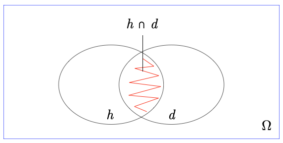
We can think of the sample space \Omega as the set of all possible outcomes in the experiment. Each point in the sample space corresponds to a unique outcome. We can draw a circle around all of the points that are described by an event, for instance that all three flips came up \text{H}. This set of points is the data (d). In this example, we condition on the event that all three flips were HEADS—meaning we restrict our attention to those outcomes. That event comprises all the outcomes (a sequence of three coin flips) where all three flips came up HEADS.

We can draw another circle around all of the points that correspond to sequences produced by the biased coin. We’ll call this set our hypothesis (h) that the coin your friend flipped was biased.

What we want to know is {P(h \mid d)}, i.e., {P(\text{biased} \mid 3~\text{H})}. This is the probability that the coin is biased given that we observed three HEADS.

Deriving Bayes’ Rule

The intersection of h and d represents all the outcomes where the biased coin was flipped and all three flips came up HEADS. We can write this probability as {P(h \cap d)}, or equivalently, P(h, d).

To find {P(h \mid d)}, we want the proportion of d’s probability that overlaps with h. This is the ratio of the probability of the intersection {h \cap d} to the total probability of d:

P(h \mid d) = \frac{P(h, d)}{P(d)}

This is the definition of conditional probability. It holds whenever {P(d) > 0}.

Algebraic rearrangement yields

P(h, d) = P(d) \, P(h \mid d)

This is the chain rule. It says that we can calculate the probability of the intersection by multiplying the total probability of d by the proportion of d that overlaps with h.

The chain rule is symmetric, so we can write both

\begin{align*} P(h, d) = P(d) \, P(h \mid d) \\ \\ P(h, d) = P(h) \, P(d \mid h) \end{align*}

It is intuitive to understand why this symmetry exists: P(a,b) is just the probability of the intersection of a and b. {a \cap b} is the same as {b \cap a}, so

{P(a,b) = P(b,a) = P(a) \, P(b \mid a) = P(b) \, P(a \mid b)}

Returning to the quantity that we want to know,

P(h \mid d) = \frac{P(h, d)}{P(d)}

Substitution of {P(h, d)} with {P(h) \; P(d \mid h)} yields

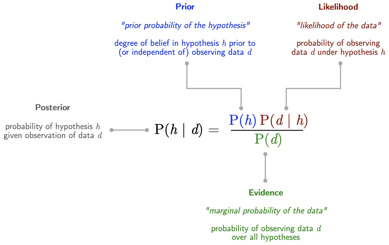
P(h \mid d) = \frac{P(h) \, P(d \mid h)}{P(d)}

This is Bayes’ rule. It follows directly from the definition of conditional probability—it is an algebraic consequence, not an additional assumption.

Why is this useful? Often we want to know the probability of a hypothesis given some observed data, P(h \mid d), but we don’t have direct access to that quantity. What we can typically specify is the likelihood—how probable the data would be under each hypothesis, P(d \mid h)—and the prior probability of each hypothesis, P(h). Bayes’ rule lets us compute the quantity we want from the quantities we have.

There are names for each of the terms.

In the case of this example:

Posterior {P(h \mid d)}: The probability that the coin is biased given that it produced the data d (a sequence of all HEADS). This is what we want to know.
Prior {P(h)}: The probability that the coin is biased before seeing any data. This is 1/10 (since there’s 1 biased coin out of 10).
Likelihood {P(d \mid h)}: The probability of getting all HEADS in 3 flips given that the coin is biased. We’ll calculate this below.
Evidence {P(d)}: The overall probability of getting all HEADS (from either coin). We’ll also calculate this below.

Applying Bayes’ Rule

On paper

Let’s now fill in our probabilities to answer the question.

We know that,

P(h) = \frac{1}{10} = 0.1

since there is 1 biased coin and 9 fair coins.

We also know that for the biased coin,

P(d \mid h) = (0.9)^3 = 0.729

since each flip independently has probability 0.9 of landing HEADS, and we need all three to be HEADS.

Additional details

More generally, the probability of getting k HEADS in n flips follows a binomial distribution:

P(k \text{ heads in } n \text{ flips}) = \binom{n}{k} \cdot p^k \cdot (1 - p)^{n-k}

In our case, k = n = 3 and p = 0.9, so \binom{3}{3} = 1 and the formula reduces to p^3. For other numbers of heads the binomial coefficient would be non-trivial—e.g., for exactly 2 HEADS in 3 flips, \binom{3}{2} = 3 because there are three distinct sequences (HHT, HTH, THH).

To calculate {P(d)}, we need to consider both the case where the coin is biased and the case where the coin is fair.

P(d) = P(h) \, P(d \mid h) + P(\neg h) \, P(d \mid \neg h)

Or more generally, when there are more than two hypotheses, we sum over the full hypothesis space \mathcal{H}:

P(d) = \sum_{h' \in \mathcal{H}} P(h') \, P(d \mid h')

For this coin example, h is the coin was biased and \neg h is the coin was fair:

\begin{align*} P(d) &= P(d, h) + P(d, \neg h) \\ &= P(h) \, P(d \mid h) + P(\neg h) \, P(d \mid \neg h) \\ &= (0.1)(0.9)^3 + (0.9)(0.5)^3 \\ &= (0.1)(0.729) + (0.9)(0.125) \\ &= 0.0729 + 0.1125 \\ &= 0.1854 \end{align*}

Finally, we can plug everything into Bayes’ rule:

\begin{align*} P(h \mid d) &= \frac{P(h) \, P(d \mid h)}{P(d)} \\ \\ &= \frac{0.1 \cdot 0.729}{0.1854} \\ \\ &\approx 0.393 \end{align*}

The probability that your friend flipped the biased coin is approximately 0.393.

Notice what happened: the prior probability of the biased coin was just 0.1, but after observing three HEADS, the posterior jumped to nearly 0.4—a roughly fourfold increase. The data was diagnostic: getting all HEADS is much more likely under the biased coin (0.729) than the fair coin (0.125), so the observation shifted our belief substantially toward the biased-coin hypothesis. The prior and likelihood together define a generative model—first a coin is drawn (prior), then flips are produced (likelihood)—and Bayes’ rule inverts this generative process to reason from observed data back to probable causes.

In the `memo` PPL

import jax
import jax.numpy as jnp
from memo import memo
from memo import domain as product
from enum import IntEnum

class Coin(IntEnum):
    TAILS = 0
    HEADS = 1

class Bag(IntEnum):
    FAIR = 0
    BIASED = 1

nflips = 3

S = product(**{f"f{flip+1}": len(Coin) for flip in range(nflips)})

NumHeads = jnp.arange(nflips + 1)

@jax.jit
def sum_seq(s):
    return S.f1(s) + S.f2(s) + S.f3(s)

@jax.jit
def pmf(s, c):
    ### probability of heads for fair and biased coin
    p_h = jnp.array([0.5, 0.9])[c]
    ### P(T) and P(H) for coin c
    p = jnp.array([1 - p_h, p_h])
    ### probability of the outcome of each flip
    p1 = p[S.f1(s)]
    p2 = p[S.f2(s)]
    p3 = p[S.f3(s)]
    ### probability of the sequence s
    return p1 * p2 * p3

@memo
def experiment[_numheads: NumHeads]():
    ### observer's mental model of the process by which
    ### the friend observed the number of heads
    observer: thinks[
        ### friend draws a coin from the bag
        friend: draws(c in Bag, wpp=0.1 if c == {Bag.BIASED} else 0.9),
        ### friend flips the coin 3x
        friend: given(s in S, wpp=pmf(s, c)),
        ### friend counts the number of HEADS
        friend: given(numheads in NumHeads, wpp=(numheads==sum_seq(s)))
    ]
    ### observer learns the number of heads from friend
    observer: observes [friend.numheads] is _numheads

    ### query the observer: what's the probability that 
    ### the coin c, which your friend flipped, was biased?
    return observer[Pr[friend.c == {Bag.BIASED}]]

xa = experiment(print_table=True, return_aux=True, return_xarray=True).aux.xarray

numheads = 3
print(f"\n\nP(h=biased | d={numheads}heads) = {xa.loc[numheads].item()}\n")

+---------------------+-----------------------+
| _numheads: NumHeads | experiment            |
+---------------------+-----------------------+
| 0                   | 0.000888100010342896  |
| 1                   | 0.007936511188745499  |
| 2                   | 0.06716419756412506   |
| 3                   | 0.39320388436317444   |
+---------------------+-----------------------+


P(h=biased | d=3heads) = 0.39320388436317444

Exercises

Imagine that your friend tells you that the coin is red. What is the probability that the sequence of three flips contains exactly 2 Heads?

In this scenario, what is the hypothesis and what is the data?
Describe (in words) the prior, likelihood, evidence and posterior for this scenario, and write out the calculations for each.

Write a memo model to infer the posterior for this scenario.

More data

Suppose your friend draws a coin and flips it 10 times, reporting 9 HEADS. Compute P(\text{biased} \mid 9\text{H in }10) using Bayes’ rule. How does the posterior compare to the 3-flip case? What does this tell you about the relationship between the amount of data and the strength of the posterior update?

Solution

\begin{align*} P(d \mid h) &= \binom{10}{9}(0.9)^9(0.1)^1 = 10 \cdot 0.3874 \cdot 0.1 \approx 0.3874 \\ P(d \mid \neg h) &= \binom{10}{9}(0.5)^{10} = 10 / 1024 \approx 0.00977 \\ P(d) &= (0.1)(0.3874) + (0.9)(0.00977) \approx 0.04753 \\ P(h \mid d) &= \frac{0.03874}{0.04753} \approx 0.815 \end{align*}

The posterior jumps from 0.1 to approximately 0.815—far more dramatic than the 3-flip case (\approx 0.393). With more data, the likelihood ratio becomes more extreme: under the biased coin, 9 heads in 10 is plausible (0.387), but under the fair coin it is very unlikely (0.010). More data allows us to discriminate more sharply between hypotheses.

Render env

%reset -f
import sys
import platform
import importlib.metadata

print("Python:", sys.version)
print("Platform:", platform.system(), platform.release())
print("Processor:", platform.processor())
print("Machine:", platform.machine())

print("\nPackages:")
for name, version in sorted(
    ((dist.metadata["Name"], dist.version) for dist in importlib.metadata.distributions()),
    key=lambda x: x[0].lower()  # Sort case-insensitively
):
    print(f"{name}=={version}")

Python: 3.14.3 (main, Feb  4 2026, 01:51:49) [Clang 21.1.4 ]
Platform: Darwin 24.6.0
Processor: arm
Machine: arm64

Packages:
altair==6.0.0
annotated-types==0.7.0
anyio==4.12.1
anywidget==0.9.21
appnope==0.1.4
argon2-cffi==25.1.0
argon2-cffi-bindings==25.1.0
arrow==1.4.0
astroid==4.0.4
asttokens==3.0.1
async-lru==2.1.0
attrs==25.4.0
babel==2.18.0
beautifulsoup4==4.14.3
bleach==6.3.0
certifi==2026.1.4
cffi==2.0.0
cfgv==3.5.0
charset-normalizer==3.4.4
click==8.3.1
colour-science==0.4.7
comm==0.2.3
contourpy==1.3.3
cycler==0.12.1
debugpy==1.8.20
decorator==5.2.1
defusedxml==0.7.1
dill==0.4.1
distlib==0.4.0
distro==1.9.0
docutils==0.22.4
executing==2.2.1
fastjsonschema==2.21.2
filelock==3.20.3
fonttools==4.61.1
fqdn==1.5.1
h11==0.16.0
httpcore==1.0.9
httpx==0.28.1
identify==2.6.16
idna==3.11
importlib_metadata==8.7.1
ipykernel==7.2.0
ipython==9.10.0
ipython_pygments_lexers==1.1.1
ipywidgets==8.1.8
isoduration==20.11.0
isort==7.0.0
itsdangerous==2.2.0
jax==0.9.0.1
jaxlib==0.9.0.1
jedi==0.19.2
Jinja2==3.1.6
jiter==0.13.0
joblib==1.5.3
json5==0.13.0
jsonpointer==3.0.0
jsonschema==4.26.0
jsonschema-specifications==2025.9.1
jupyter-cache==1.0.1
jupyter-events==0.12.0
jupyter-lsp==2.3.0
jupyter_client==8.8.0
jupyter_core==5.9.1
jupyter_server==2.17.0
jupyter_server_terminals==0.5.4
jupyterlab==4.5.3
jupyterlab_pygments==0.3.0
jupyterlab_server==2.28.0
jupyterlab_widgets==3.0.16
kiwisolver==1.4.9
lark==1.3.1
marimo==0.19.9
Markdown==3.10.1
MarkupSafe==3.0.3
matplotlib==3.10.8
matplotlib-inline==0.2.1
mccabe==0.7.0
memo-lang==1.2.9
mistune==3.2.0
ml_dtypes==0.5.4
msgspec==0.20.0
narwhals==2.16.0
nbclient==0.10.4
nbconvert==7.17.0
nbformat==5.10.4
nest-asyncio==1.6.0
networkx==3.6.1
nodeenv==1.10.0
notebook_shim==0.2.4
numpy==2.4.2
numpy-typing-compat==20251206.2.4
openai==2.17.0
opt_einsum==3.4.0
optype==0.15.0
packaging==26.0
pandas==3.0.0
pandas-stubs==3.0.0.260204
pandocfilters==1.5.1
parso==0.8.5
pexpect==4.9.0
pillow==12.1.0
platformdirs==4.5.1
plotly==5.24.1
pre_commit==4.5.1
prometheus_client==0.24.1
prompt_toolkit==3.0.52
psutil==7.2.2
psygnal==0.15.1
ptyprocess==0.7.0
pure_eval==0.2.3
pycparser==3.0
pydantic==2.12.5
pydantic_core==2.41.5
Pygments==2.19.2
pygraphviz==1.14
pylint==4.0.4
pymdown-extensions==10.20.1
pyparsing==3.3.2
python-dateutil==2.9.0.post0
python-dotenv==1.2.1
python-json-logger==4.0.0
PyYAML==6.0.3
pyzmq==27.1.0
referencing==0.37.0
requests==2.32.5
rfc3339-validator==0.1.4
rfc3986-validator==0.1.1
rfc3987-syntax==1.1.0
rpds-py==0.30.0
ruff==0.15.0
scikit-learn==1.8.0
scipy==1.17.0
scipy-stubs==1.17.0.2
seaborn==0.13.2
Send2Trash==2.1.0
setuptools==81.0.0
six==1.17.0
sniffio==1.3.1
soupsieve==2.8.3
SQLAlchemy==2.0.46
stack-data==0.6.3
starlette==0.52.1
tabulate==0.9.0
tenacity==9.1.4
terminado==0.18.1
threadpoolctl==3.6.0
tinycss2==1.4.0
toml==0.10.2
tomlkit==0.14.0
tornado==6.5.4
tqdm==4.67.3
traitlets==5.14.3
typing-inspection==0.4.2
typing_extensions==4.15.0
tzdata==2025.3
uri-template==1.3.0
urllib3==2.6.3
uvicorn==0.40.0
virtualenv==20.36.1
wcwidth==0.6.0
webcolors==25.10.0
webencodings==0.5.1
websocket-client==1.9.0
websockets==16.0
widgetsnbextension==4.0.15
xarray==2026.1.0
zipp==3.23.0

References

Ma, Wei Ji, Kording, Konrad, & Goldreich, Daniel. (2023). Bayesian models of perception and action: An introduction. The MIT Press.