Recursive Beliefs

Thinking about thinking with the 2/3rds game

Inspired by: Nagel (1995), “Unraveling in guessing games: An experimental study”.

Imagine that a newspaper like the New York Times runs a contest. Readers can write in a guess of an integer from 0-100. The editor computes the average of the readers’ guesses. The winner is the reader whose guess is closest to 2/3rds of the average.

Before continuing, write down what you would guess!

After you’ve written down your guess for (i) the New York Times readers, write down your guess if you were playing this game with (ii) a group of your friends, and (iii) a group of economists.

Are you guesses for (i), (ii), and (iii) the same? Different?

This problem evokes recursive reasoning over a Theory of Mind. One way to make a guess is to reason about what other people would reason about other people’s reasoning.

The Nash equilibrium for this game is for all readers to guess 0 or 1. However, in practice most people guess a number much higher than that. Why?

One reason a reader might choose a higher number is that she expects others to be less rational, and so they will on average pick a number greater than 2. It could also be that a reader thinks that others are rational enough to choose 0 or 1, but thinks that those people believe other people are less rational. Or maybe the reader was just not able to find the Nash equilibrium herself.

In this tutorial, we will model a “level-k” strategy for this game, and then fit the model’s predictions to real data collected by the New York Times.

Let’s bring in some of the standard imports.

import jax
import jax.numpy as jnp
from memo import memo
from matplotlib import pyplot as plt

Readers can choose an integer between 0 and 100, inclusive. Let’s define that sample space N.

N = jnp.arange(100 + 1)
N.shape

(101,)

A good practice for writing probabilistic models is to start with an overly simplified model and then build up. We’ll start with a generative model of what choices the greater population of readers make. Recall how we modeled dice rolls in the Generative Models 1 tutorial. Let’s start by building a generative model of a uniformly random draw from this sample space (like rolling a 101-sided die).

@memo
def d101[_n: N]():
    observer: draws(n in N, wpp=1)
    return Pr[observer.n == _n]

d101()

Array([0.00990099, 0.00990099, 0.00990099, 0.00990099, 0.00990099,
       0.00990099, 0.00990099, 0.00990099, 0.00990099, 0.00990099,
       0.00990099, 0.00990099, 0.00990099, 0.00990099, 0.00990099,
       0.00990099, 0.00990099, 0.00990099, 0.00990099, 0.00990099,
       0.00990099, 0.00990099, 0.00990099, 0.00990099, 0.00990099,
       0.00990099, 0.00990099, 0.00990099, 0.00990099, 0.00990099,
       0.00990099, 0.00990099, 0.00990099, 0.00990099, 0.00990099,
       0.00990099, 0.00990099, 0.00990099, 0.00990099, 0.00990099,
       0.00990099, 0.00990099, 0.00990099, 0.00990099, 0.00990099,
       0.00990099, 0.00990099, 0.00990099, 0.00990099, 0.00990099,
       0.00990099, 0.00990099, 0.00990099, 0.00990099, 0.00990099,
       0.00990099, 0.00990099, 0.00990099, 0.00990099, 0.00990099,
       0.00990099, 0.00990099, 0.00990099, 0.00990099, 0.00990099,
       0.00990099, 0.00990099, 0.00990099, 0.00990099, 0.00990099,
       0.00990099, 0.00990099, 0.00990099, 0.00990099, 0.00990099,
       0.00990099, 0.00990099, 0.00990099, 0.00990099, 0.00990099,
       0.00990099, 0.00990099, 0.00990099, 0.00990099, 0.00990099,
       0.00990099, 0.00990099, 0.00990099, 0.00990099, 0.00990099,
       0.00990099, 0.00990099, 0.00990099, 0.00990099, 0.00990099,
       0.00990099, 0.00990099, 0.00990099, 0.00990099, 0.00990099,
       0.00990099], dtype=float32)

Modeling agentic choice

We’re now going to rewrite the program in the mentalistic grammar of memo. memo provides several random-variable-constructor verbs: chooses, given, draws, assigned, guesses. These are functionally identical (they alias to the same internal function), but their semantics allow us to make different epistemological expressions. Since we think that people are intentionally choosing a number, let’s replace draws() with chooses(). We’ll also update the function name and the agent to reflect what we’re modeling, renaming observer to population and the model to population_uniform_choice.

@memo
def population_uniform_choice[_n: N]():
    population: chooses(n in N, wpp=1)
    return Pr[population.n == _n]

### prove to ourselves that these models give the same output
jnp.array_equal(population_uniform_choice(), d101()).item()

True

Parametric priors

Let’s add a bit of complexity. Say that we think that people’s choice of numbers is Gaussian rather than uniform. We can add a prior by passing a probability function as wpp. We’ll start with distribution centered at 50 and give it a standard deviation of 3.

from jax.scipy.stats.norm import pdf as normpdf

@memo
def population_gaussian_choice[_n: N]():
    population: chooses(
        n in N,
        wpp=normpdf(n, loc=50, scale=3)
    )
    return Pr[population.n == _n]

res = population_gaussian_choice()
expectation = jnp.dot(res, N).item()

fig, ax = plt.subplots()
_ = ax.bar(N, res)
_ = ax.set_xticks(range(0, 100 + 1, 10))
_ = ax.axvline(
    expectation,
    color="black",
    linestyle="--",
    alpha=0.8,
    label=r"$\mathbf{E}[\mathtt{population.\!\!n}] = " + f"{expectation:.2f}$")
_ = ax.set_xlabel("$\mathtt{population.\!\!n}$")
_ = ax.set_ylabel("Probability")
_ = ax.legend()
print(f"Expectation: {expectation}")

Expectation: 50.0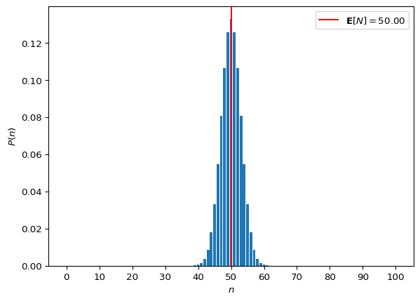

Try playing with the parameters of the prior. We know that Gaussian distributions are symmetric. When the distribution is centered on 50, the expectation of the choices is 50 (that makes sense). What happens if you use \mathcal{N}(\mu=5, \sigma=3)? What about \mu=0?

Probability functions

In this example, we are passing a probability density function (PDF) as wpp. memo will treat this as a probability mass function (PMF), normalizing the probability density measure over the discrete support.

For instance, \sum_{x \in \{0, 2, 4\}} \mathcal{N}(x \mid \mu{=}0, \sigma{=}1) is, of course, not going to to form a proper probability measure (it does not sum to one):

X = jnp.array([0, 2, 4])

print(f"Sum: {normpdf(X, loc=0, scale=1).sum()}")

Sum: 0.4530670940876007

But when passed as wpp, memo converts these values into a PMF.

@memo
def example[_x: X]():
    a: chooses(
        x in X,
        wpp=normpdf(x, loc=0, scale=1)
    )
    return Pr[a.x == _x]

example()

print(f"Sum: {example().sum()}")

Array([8.8053691e-01, 1.1916769e-01, 2.9538717e-04], dtype=float32)

Sum: 1.0

Enumeration over query variables

Query variables

In the definition of a @memo, you can include “query variables” in square brackets, e.g. def f[_a: A, _b: B, _c: C]():. memo will enumerate over the values that these can take, returning an array with the same number of axes.

A = (jnp.arange(2) + 1) * 100
B = (jnp.arange(3) + 1) * 10
C = jnp.arange(4) + 1

@memo
def f[_a: A, _b: B, _c: C]():  ### Specify the query variables in the function definition
    return _a + _b + _c  ### Return the sum of the query variables

f()
print(f"Shape of output array: {f().shape}")

Array([[[111, 112, 113, 114],
        [121, 122, 123, 124],
        [131, 132, 133, 134]],

       [[211, 212, 213, 214],
        [221, 222, 223, 224],
        [231, 232, 233, 234]]], dtype=int32)

Shape of output array: (2, 3, 4)

The @memo f() above will enumerate over \{ (\_a, \_b, \_c) : \_a \in A, \_b \in B, \_c \in C \}. This causes @memo to return an array with 3 axes, where each element is the value of the @memo evaluated at the query variables jointly: f(_a, _b, _c). Thus, f() outputs an array with 3 axes (corresponding to _a, _b, and _c), where dimension 1 has a size of len(A) (the number of element in A, which is 2), dimension 2 has a size of len(B), and dimension 3 has a size of len(C).

This is easy to see with print_table=True:

_ = f(print_table=True)

+-------+-------+-------+------+
| _a: A | _b: B | _c: C | f    |
+-------+-------+-------+------+
| 100   | 10    | 1     | 111  |
| 100   | 10    | 2     | 112  |
| 100   | 10    | 3     | 113  |
| 100   | 10    | 4     | 114  |
| 100   | 20    | 1     | 121  |
| 100   | 20    | 2     | 122  |
| 100   | 20    | 3     | 123  |
| 100   | 20    | 4     | 124  |
| 100   | 30    | 1     | 131  |
| 100   | 30    | 2     | 132  |
| 100   | 30    | 3     | 133  |
| 100   | 30    | 4     | 134  |
| 200   | 10    | 1     | 211  |
| 200   | 10    | 2     | 212  |
| 200   | 10    | 3     | 213  |
| 200   | 10    | 4     | 214  |
| 200   | 20    | 1     | 221  |
| 200   | 20    | 2     | 222  |
| 200   | 20    | 3     | 223  |
| 200   | 20    | 4     | 224  |
| 200   | 30    | 1     | 231  |
| 200   | 30    | 2     | 232  |
| 200   | 30    | 3     | 233  |
| 200   | 30    | 4     | 234  |
+-------+-------+-------+------+

Details and examples

In the process of building up a model, you might start with something like this, which doesn’t have any query variables.

X = jnp.array([40, 45, 55, 60])
@memo
def example1():
    agent: chooses(x in X, wpp=1)
    return Pr[agent.x]
res = example1()
print(f"Shape: {res.shape}")
res

Shape: ()

Array(50., dtype=float32)

What’s being returned by example1()?

Since there are no query variables, the function will always return the same value. In this case, it’s the expectation of the agent’s choice. To see the probability of each choice x, enumerate over \{\_x \in X\} and return the probability for each \_x.

X = jnp.array([40, 45, 55, 60])
@memo
1def example2[_x: X]():
    agent: chooses(x in X, wpp=1)
2    return Pr[agent.x == _x]
res = example2()
print(f"Mean: {res.mean()}")
print(f"Expectation: {jnp.dot(res, X)}")
print(f"Shape: {res.shape}")
res

1: Add [_x: X] to the function definition
2: Add == _x to the return statement

Mean: 0.25
Expectation: 50.0
Shape: (4,)

Array([0.25, 0.25, 0.25, 0.25], dtype=float32)

Adding [_x: X] to the function definition makes memo add a new dimension to the output data. Adding == _x to the return statement makes the function return a value (in this case, the probability that the agent chooses _x) for each value of _x.

Notice that def example1(): returns Array(50.), which has the shape () (i.e. no dimensions, it is a single number). However, def example2[_x: X](): returns Array([0.25, 0.25, 0.25, 0.25]), which has the shape (4,) (i.e. an array with one axis and 4 elements).

In this way, you can evaluate a @memo for multiple query variables jointly:

from enum import IntEnum

A = jnp.arange(3) * -1

class B(IntEnum):
    VAL1 = 0
    VAL2 = 1

C = jnp.arange(4) + 100

@memo
def example3[_a: A, _b: B, _c: C]():
    agent: chooses(a in A, wpp=1)
    agent: chooses(b in B, wpp=1)
    agent: chooses(c in C, wpp=1)
    return Pr[agent.a == _a, agent.b == _b, agent.c == _c]

res = example3(print_table=True)
print(f"Shape: {res.shape}")
res

+-------+-------+-------+---------------------+
| _a: A | _b: B | _c: C | example3            |
+-------+-------+-------+---------------------+
| 0     | VAL1  | 100   | 0.0416666679084301  |
| 0     | VAL1  | 101   | 0.0416666679084301  |
| 0     | VAL1  | 102   | 0.0416666679084301  |
| 0     | VAL1  | 103   | 0.0416666679084301  |
| 0     | VAL2  | 100   | 0.0416666679084301  |
| 0     | VAL2  | 101   | 0.0416666679084301  |
| 0     | VAL2  | 102   | 0.0416666679084301  |
| 0     | VAL2  | 103   | 0.0416666679084301  |
| -1    | VAL1  | 100   | 0.0416666679084301  |
| -1    | VAL1  | 101   | 0.0416666679084301  |
| -1    | VAL1  | 102   | 0.0416666679084301  |
| -1    | VAL1  | 103   | 0.0416666679084301  |
| -1    | VAL2  | 100   | 0.0416666679084301  |
| -1    | VAL2  | 101   | 0.0416666679084301  |
| -1    | VAL2  | 102   | 0.0416666679084301  |
| -1    | VAL2  | 103   | 0.0416666679084301  |
| -2    | VAL1  | 100   | 0.0416666679084301  |
| -2    | VAL1  | 101   | 0.0416666679084301  |
| -2    | VAL1  | 102   | 0.0416666679084301  |
| -2    | VAL1  | 103   | 0.0416666679084301  |
| -2    | VAL2  | 100   | 0.0416666679084301  |
| -2    | VAL2  | 101   | 0.0416666679084301  |
| -2    | VAL2  | 102   | 0.0416666679084301  |
| -2    | VAL2  | 103   | 0.0416666679084301  |
+-------+-------+-------+---------------------+
Shape: (3, 2, 4)

Array([[[0.04166667, 0.04166667, 0.04166667, 0.04166667],
        [0.04166667, 0.04166667, 0.04166667, 0.04166667]],

       [[0.04166667, 0.04166667, 0.04166667, 0.04166667],
        [0.04166667, 0.04166667, 0.04166667, 0.04166667]],

       [[0.04166667, 0.04166667, 0.04166667, 0.04166667],
        [0.04166667, 0.04166667, 0.04166667, 0.04166667]]], dtype=float32)

Indexing output

Remember that you can convert these into an pandas DataFrame or an xarray for easy indexing, e.g. xa.loc[-2, "VAL2", 103]:

res = example3(return_xarray=True)
data = res.data
xa = res.aux.xarray
print(f"JAX array:   {data[2, 1, 3]}")
print(f"xarray:      {xa.loc[-2, "VAL2", 103].item()}")

JAX array:   0.0416666679084301
xarray:      0.0416666679084301

Empty axes

If you include a query variable in the function definition, but return a value that does not depend on the query variable, memo will add an empty axis to the output array:

@memo
def example4[_a: A, _b: B, _c: C]():
    agent: chooses(a in A, wpp=1)
    agent: chooses(b in B, wpp=1)
    agent: chooses(c in C, wpp=1)
    # return Pr[agent.a == _a, agent.b == _b, agent.c == _c]
    return Pr[agent.b == _b]

res = example4()
print(f"Shape: {res.shape}")
res

Shape: (1, 2, 1)

Array([[[0.5],
        [0.5]]], dtype=float32)

Identity of query variables

Note that multiple query variables can derive from the same sample space, as in \{\_x \in Z\} and \{\_y \in Z\}.

C = jnp.arange(-10, 10+1)
Z = jnp.array([-1, 0, 1])

@memo
def example5[_x: Z, _y: Z]():
    agent1: chooses(c in C, wpp=1)
    agent2: chooses(c in C, wpp=1)
    return Pr[agent1.c < _x, agent2.c > _y]

res = example5()
print(f"Shape: {res.shape}")
res

Shape: (3, 3)

Array([[0.22448967, 0.20408155, 0.18367343],
       [0.24943294, 0.22675724, 0.20408155],
       [0.2743762 , 0.24943294, 0.22448967]], dtype=float32)

Using a `@memo` as a submodel

Returning to our example, we have a simple generative model of the populations’ choice. Let’s now model a reader thinking about the population. We can do this with the memo syntax thinks[...]. In the model below, we build a new @memo, reader_thinks() with a new mental frame, reader.

@memo
def population_gaussian_choice_wpp[_n: N]():
    population: chooses(n in N, wpp=normpdf(n, 50, 3))
    return Pr[population.n == _n]

@memo
def reader_thinks():
    reader: thinks[
        population: chooses(
            n in N,
            wpp=population_gaussian_choice_wpp[n]()
        )
    ]
    return reader[ E[population.n] ]

reader_thinks()

Array(50., dtype=float32)

The reader_thinks() model simulates what number the reader thinks the population will choose, resulting in a probability for each of the 101 numbers. This probability represents the reader’s graded beliefs about the population’s choice. Then, the @memo returns the reader’s expectation (the reader’s averaged belief) of the population’s choice (return reader[ E[population.n] ]).

Pay attention to the grammar here: reader[ ... ] means that we are querying information in the reader’s mind. Specifically, the reader’s expectation (E[ ... ]) of the population’s choice n. Square brackets function as a way of entering a mental frame.¹

Technical aside

We are now using E (for Expectation) rather than Pr (for Probability).

E and Pr are closely related. For a boolean condition C, the probability P(C) equals the expectation of the indicator function: P(C) = E[\mathbf{1}_C]. In memo, Pr[condition] computes exactly this—the expectation of the indicator that evaluates to 1 when the condition is true and 0 otherwise. This is why the two operators can often be used interchangeably.

Notice how the @memo “population_gaussian_choice_wpp()” is serving as a submodel in the @memo “reader_thinks()”. We’ll return to this idea shortly. For the moment, since there’s nothing complicated happening in population_gaussian_choice_wpp(), let’s simplify the model into a single @memo:

@memo
def reader_thinks():
    reader: thinks[
        population: chooses(n in N, wpp=normpdf(n, 50, 3))  ### inline population_gaussian_choice_wpp[n]()
    ]
    return reader[ E[population.n] ]  ### query what the reader thinks about the population

reader_thinks()

Array(50., dtype=float32)

And just to make the next steps as clear as possible, let’s return to a uniform prior over the reader’s belief about the population’s choice:

@memo
def reader_thinks():
    reader: thinks[
        population: chooses(n in N, wpp=1)  ### back to a uniform prior
    ]
    return reader[ E[population.n] ]  ### query what the reader thinks about the population

reader_thinks()

Array(50., dtype=float32)

Encapsulation in mental frames

A key design principle of memo is encapsulation, meaning that information is bound to “frames”. To be accessible outside of its frame, encapsulated information must be explicitly exposed.

The population frame only exists within the reader’s mind. I.e. population is a representation internal to the reader mental frame. Trying to access the population frame outside of the reader frame raises an error.

@memo
def psychic_reader():
    reader: thinks[
        population: chooses(n in N, wpp=1)
    ]
    # return reader[ E[population.n] ]  ### query what the reader thinks about the population
    #########
    ### attempt to access information about the
    ### population outside of the reader's mind:
    #########
    return E[population.n]
psychic_reader()

memo.core.MemoError: Unknown choice population.n
  file: "1969463279.py", line 11, in @memo psychic_reader
        return E[population.n]
                 ^

  hint: Did you perhaps misspell n? population is not yet aware of any
        choice called n. Or, did you forget to call
        population.chooses(n ...) or population.knows(n) earlier in
        the memo?

  ctxt: This error was encountered in the frame of population.  In
        that frame, population is currently modeling the following 0
        choices: .

  info: You are using memo 1.2.9, JAX 0.8.2, Python 3.14.2 on Darwin.

The memo language forces us to specify that we are modeling what the reader thinks about the population, and that this is different than the actual population (which we are not currently modeling).

Choice based on mental simulation

Let’s model the reader actually playing the game (in the most simple way possible). Rather than the reader estimating the average of the population’s choice, we’ll have the reader estimate 2/3rds of the average.

@memo
def reader_thinks():
    reader: thinks[
        population: chooses(n in N, wpp=1)
    ]
    return reader[ (2/3)*E[population.n] ]

reader_thinks()

Array(33.333336, dtype=float32)

Now that the reader is estimating 2/3rds of the population’s average choice, we can model the reader’s choice. We’ll start by modeling the reader as perfectly rational. I.e. the reader will always pick the value that’s closest to 2/3rds of what the reader thinks the population’s average choice will be.

To accomplish this perfectly rational behavior, replace wpp in chooses(...) with to_minimize. The to_minimize keyword causes chooses() to perform an \mathrm{argmin}, assigning a probability of 1 to the choice with the lowest weight and zero to everything else.

To have the reader pick the choice closest to 2/3rds the average, we find the absolute difference between 2/3rds the average and every possible choice (n) that the reader could make:

abs( (2/3)*E[population.n] - n )

We tell memo to pick the n associated with the lowest value via to_minimize=....²

@memo
def reader_choice[_n: N]():
    reader: thinks[
        population: chooses(n in N, wpp=1)
    ]

    reader: chooses(
        n in N, 
        to_minimize=abs( (2/3)*E[population.n] - n )
    )
    return Pr[reader.n == _n]

jnp.where(reader_choice())

(Array([33], dtype=int32),)

Frame context in agent statements

Notice that the reader: chooses(...) statement uses E[population.n] directly whereas the reader_thinks() model’s return statement (reader[ (2/3)*E[population.n] ]) has an additional set of brackets: reader[...]. Why?

An agent only has access to her own mental contents so only things within her mental frame can affect her choice. When we write reader: chooses(...), we are entering the reader’s mental frame. The reader: prefix establishes that this choice is made from the reader’s perspective, using only information available to the reader. Since population is represented by the reader (it is defined in the reader: thinks[...] block), the reader can access E[population.n] directly.

Contrast this with return statements, which execute from the root frame. To access the reader’s beliefs from the root frame, we must explicitly enter the reader’s frame using reader[...].

The model returns the probability of the reader making each choice. Since we’re using to_minimize, the reader will always choose the n with the smallest absolute error, so evaluating reader_choice() produces an array of len(N) elements, with all of the probability mass on the n closest to (2/3)*E[population.n].

jnp.where(...) returns the indices at which there are non-zero values. Is this the index you expect?

Under a uniform prior, the expected value of the population’s choice is 50. 2/3rds of that is 33.3333. The closest n that the reader can choose is 33, which is index 33 in N. It seems this model does what we expect it to, but it is still far from being a model of what we think readers are actually doing.

Recursive reasoning

A critical missing component is the reader thinking about other readers who are also thinking about what other readers think about other readers. How can we model this recursive reasoning?

We previously saw how a @memo can be used as a probability function in the chooses() statement of another @memo.

Let’s re-write the model above using a submodel:

@memo
def population_uniform_choice_wpp[_n: N]():
    population: chooses(n in N, wpp=1)
    return Pr[population.n == _n]

@memo
def reader_choice_k0[_n: N]():
    reader: thinks[
        population: chooses(n in N, wpp=population_uniform_choice_wpp[n]())
    ]

    reader: chooses(
        n in N, 
        to_minimize=abs( (2/3)*E[population.n] - n )
    )
    return Pr[reader.n == _n]

jnp.where(reader_choice_k0())

(Array([33], dtype=int32),)

Notice that both population_uniform_choice_wpp() and reader_choice_k0() return a distribution over N. To model reader reasoning about how a population of readers would choose a number, we can replace population_uniform_choice_wpp in reader_choice_k0 with reader_choice_k0 itself:

@memo
def reader_choice_k0[_n: N]():
    reader: thinks[population: chooses(n in N, wpp=reader_choice_k0[n]())]
    ...

Thus, every time reader_choice_k0() runs, it asks reader_choice_k0() for the distribution P(\,population.\!\!n\,). This will go on ad infinitum (or until your runaway program bumps into a guardrail, see “Bottomless recursion” below). To make the recursion finite and tractable, let’s give it a bottom.

@memo
1def reader_choice_k[_n: N](k):
    reader: thinks[
        population: chooses(
            n in N,
2            wpp=reader_choice_k[n](k=k-1) if k > 0 else 1
        )
    ]

    reader: chooses(
        n in N, 
        to_minimize=abs( (2/3)*E[population.n] - n )
    )
    return Pr[reader.n == _n]

3jnp.where(reader_choice_k(k=1))

1: Pass a k level to the @memo (reader_choice_k) as an argument
2: Evaluate reader_choice_k(k=k-1) to get a probability measure for each n
3: Evaluate the model for a level-k 1 reader.

(Array([22], dtype=int32),)

The reader_choice_k model makes two changes to the reader_choice_k0 model. First, the function definition is modified: An integer k is passed to the model as an argument. Notice that this is different than a query variable (e.g. [_n: N]). Whereas _n is bound to the outer frame (i.e. the frame of the reader_choice_k function), the k argument is unbound and can be accessed anywhere in the @memo. Second, the probability that (in the reader’s mind) the population will choose n is given by reader_choice_k[n](k=k-1) if k > 0 else 1. Let’s break this down.

reader_choice_k is defined with [_n: N], which specifies that it should enumerate over \_n \in N. When reader_choice_k is called in population: chooses(n in N, wpp=...), the n being considered is passed reader_choice_k as _n: reader_choice_k[n]. This is how the probability for the correct value of n is passed as wpp. The function also needs to be called, using (...). If there are no arguments, then nothing goes into the parentheses (as was the case with wpp=population_gaussian_choice_wpp[n]() above). In this case, we need to pass a value for k. But what value?

We pass the submodel a k level one less than k level of the model that calls it. Why? Here’s two way to think about it: - If k does not decrease, then then recursion never terminates (you can try this if you want; replace k-1 with k and you’ll receive a RecursionError: maximum recursion depth exceeded). - To model a certain level of strategic sophistication, your cognitive system must have at least that much complexity. To represent level-k reasoning, a cognitive system must be at least level k+1.

Finally, there is a boundary condition that says “if k is 0, then treat the population as making a uniform choice”:

reader_choice_k[n](k=k-1) if k > 0 else 1

Bottomless recursion

First run this @memo as is. @memo(debug_trace=True) will produce an execution trace that shows how memo recurses through the k values.

Then try changing k-1 to k. What happens and why?

@memo(debug_trace=True)
def reader_choice_k_example[_n: N](k):
    reader: thinks[
        population: chooses(
            n in N,
            ### change from k-1 to k
            wpp=reader_choice_k_example[n](k=k-1) if k > 0 else 1
        )
    ]
    reader: chooses(n in N, to_minimize=abs( (2/3)*E[population.n] - n) )
    return Pr[reader.n == _n]

reader_choice_k_example(k=3)

 --> reader_choice_k_example(3)
 --> reader_choice_k_example(2)
 --> reader_choice_k_example(1)
 --> reader_choice_k_example(0)
<--  reader_choice_k_example(0) has shape (101,)
     time = 0.050100 sec
<--  reader_choice_k_example(1) has shape (101,)
     time = 0.050190 sec
<--  reader_choice_k_example(2) has shape (101,)
     time = 0.050253 sec
<--  reader_choice_k_example(3) has shape (101,)
     time = 0.050355 sec

Array([0., 0., 0., 0., 0., 0., 0., 0., 0., 0., 1., 0., 0., 0., 0., 0., 0.,
       0., 0., 0., 0., 0., 0., 0., 0., 0., 0., 0., 0., 0., 0., 0., 0., 0.,
       0., 0., 0., 0., 0., 0., 0., 0., 0., 0., 0., 0., 0., 0., 0., 0., 0.,
       0., 0., 0., 0., 0., 0., 0., 0., 0., 0., 0., 0., 0., 0., 0., 0., 0.,
       0., 0., 0., 0., 0., 0., 0., 0., 0., 0., 0., 0., 0., 0., 0., 0., 0.,
       0., 0., 0., 0., 0., 0., 0., 0., 0., 0., 0., 0., 0., 0., 0., 0.],      dtype=float32)

What happens when we pass this model different k values?

for k_ in range(12):
    res = reader_choice_k(k=k_)
    print(f"k = {k_:>2}   ->   guess = {jnp.where(res)[0].item():>2}")

k =  0   ->   guess = 33
k =  1   ->   guess = 22
k =  2   ->   guess = 15
k =  3   ->   guess = 10
k =  4   ->   guess =  7
k =  5   ->   guess =  5
k =  6   ->   guess =  3
k =  7   ->   guess =  2
k =  8   ->   guess =  1
k =  9   ->   guess =  1
k = 10   ->   guess =  1
k = 11   ->   guess =  1

At k=0, the reader thinks that the population is making a uniform choice. Thus, the expectation is 50, and the reader guesses 33. At k=1, the reader thinks that everyone else is reasoning like the k=0 model. Thus the reader guesses 2/3rds of 33. Etc.

Why does the guess never reach zero? Remember that the reader can only choose integers. When the reader thinks that everyone else will guess 1, the model finds the integer closest to (2/3)*E[1], which is 2/3. And 0.6667 is closer to 1 than to 0, so according to this model, a perfectly rational agent will always guess 1.

Try changing (2/3) to something lower, like 0.49. What happens then? How does that change the equilibrium? Does that affect the number of steps required for the model to converge to the equilibrium?

Approximately rational choice

The reader_choice_k model assumes perfect rationality: given their beliefs about others, readers always choose the single best response. But human decision-making is noisy. People sometimes make mistakes, or they may not fully optimize.

The softmax decision rule provides a simple model of approximately rational choice (Luce, 1959). Rather than deterministically selecting the action with the best outcome, a softmax agent selects actions with probability proportional to their value. Actions with higher value are more likely to be chosen, but lower-value actions still have some probability.

Why model imperfect rationality? One goal of computational cognitive science is to infer the beliefs and preferences of agents from their observed choices. If we assume agents are perfectly rational, we can only explain behavior that exactly matches optimal play. A softmax model allows us to fit graded patterns of choice—capturing both the central tendency (what people usually do) and the variability (the range of choices people make).

Softmax

P(i) = \frac{e^{\beta \cdot z_i}}{\sum_{j} e^{\beta \cdot z_j} }

In practice we’re most often concerned with the relative probabilities of the options, so it is sufficient to use

P(i) \propto \exp(\beta z_i)

since the dominator cancels out, e.g. P(i=1)/P(i=2) = \frac{\exp(\beta \cdot z_{i=1})}{\exp(\beta \cdot z_{i=2})}.

Interactive exploration of the softmax function

In this plot, the options and corresponding values are A=1, B=0.4, and C=0 (shown in green). The probability of choosing A, B or C is shown in blue. As \beta gets larger, it becomes increasing probable that the option with the highest value (in this case, A) will be selected over the other options. In the limit of \beta approaching infinity, the softmax becomes the argmax, meaning that the option with the highest value will always be chosen, regardless of how infinitesimally smaller the value of the next best choice is.

Plotting code

import altair as alt
import pandas as pd
import numpy as np

def _softmax(x, beta=1.0):
    """Compute softmax values with inverse temperature parameter beta"""
    x = np.array(x) * beta
    exp_x = np.exp(x - np.max(x))
    return exp_x / exp_x.sum()

def make_softmax_chart(input_values, labels, y_domain, param_name='beta_val'):
    """Create an interactive Altair softmax chart with pre-computed data."""
    beta_values = [round(b, 2) for b in np.arange(0, 5.05, 0.05)]

    rows = []
    for beta in beta_values:
        probs = _softmax(input_values, beta)
        for label, val, prob in zip(labels, input_values, probs):
            rows.append({'beta': beta, 'label': label, 'type': 'Input Value', 'value': val})
            rows.append({'beta': beta, 'label': label, 'type': 'Probability', 'value': prob})

    df = pd.DataFrame(rows)

    beta_slider = alt.binding_range(min=0, max=5.0, step=0.05, name='beta: ')
    beta_param = alt.param(name=param_name, value=1.0, bind=beta_slider)

    chart = alt.Chart(df).transform_filter(
        alt.datum.beta == beta_param
    ).mark_bar().encode(
        x=alt.X('label:N', title='Option', sort=labels),
        xOffset=alt.XOffset('type:N', sort=['Input Value', 'Probability']),
        y=alt.Y('value:Q', title='Value / Probability', scale=alt.Scale(domain=y_domain)),
        color=alt.Color('type:N', scale=alt.Scale(
            domain=['Input Value', 'Probability'],
            range=['rgba(76, 175, 80, 0.7)', 'rgba(33, 150, 243, 0.7)']
        ), title='Type')
    ).add_params(
        beta_param
    ).properties(
        width=400,
        height=300,
        title='Softmax Function Demonstration'
    )

    return chart

_ = alt.data_transformers.disable_max_rows()

chart_softmax_1 = make_softmax_chart(
    input_values=[1.0, 0.4, 0.0],
    labels=['A', 'B', 'C'],
    y_domain=[0, 1.2],
    param_name='beta_val_1'
)
chart_softmax_1

The softmax function works with any real-valued input. The input values can be greater than 1, less than zero, etc.

Plotting code

chart_softmax_2 = make_softmax_chart(
    input_values=[-1.5, 0.0, 0.2],
    labels=['A', 'B', 'C'],
    y_domain=[-1.7, 1.2],
    param_name='beta_val_2'
)
chart_softmax_2

Interactive exploration softmax parameter in the game

@memo
def reader_choice_k_soft[_n: N](k, beta=1):
    reader: thinks[
        population: chooses(
            n in N,
            wpp=reader_choice_k_soft[n](k=k-1, beta=beta) if k > 0 else 1
        )
    ]
    reader: chooses(n in N, wpp=exp(beta * -abs( (2/3)*E[population.n] - n )))
    return Pr[reader.n == _n]

Plotting code

import altair as alt
import pandas as pd
import numpy as np

# Pre-compute all combinations
N_np = np.array(N)
k_values = range(0, 11)
beta_values = [round(b, 2) for b in np.arange(0, 3.05, 0.05)]

rows = []
for k in k_values:
    for beta in beta_values:
        probs = np.array(reader_choice_k_soft(k=k, beta=beta))
        mean_val = np.sum(N_np * probs)
        for n, p in zip(N_np, probs):
            rows.append({'k': k, 'beta': beta, 'n': int(n), 'prob': float(p), 'mean': mean_val, 'two_thirds_mean': mean_val * 2/3})

df_all = pd.DataFrame(rows)

# Disable max rows check for large pre-computed dataset
alt.data_transformers.disable_max_rows()

# Create Altair chart with sliders
k_slider = alt.binding_range(min=0, max=10, step=1, name='k: ')
beta_slider = alt.binding_range(min=0, max=3.0, step=0.05, name='beta: ')

k_param = alt.param(name='k_val', value=0, bind=k_slider)
beta_param = alt.param(name='beta_val', value=0.1, bind=beta_slider)

# Filter data based on slider values
base = alt.Chart(df_all).transform_filter(
    (alt.datum.k == k_param) & (alt.datum.beta == beta_param)
)

# Bar chart
bars = base.mark_bar(color='steelblue').encode(
    x=alt.X('n:Q', title='N', scale=alt.Scale(domain=[0, 100])),
    y=alt.Y('prob:Q', title='Probability', scale=alt.Scale(domain=[0, 0.2]))
)

# Mean line
mean_line = base.mark_rule(color='black', strokeWidth=2, strokeDash=[4, 4], opacity=0.5).encode(
    x='mean:Q'
)

# 2/3 Mean line
two_thirds_line = base.mark_rule(color='red', strokeWidth=2, strokeDash=[4, 4], opacity=0.5).encode(
    x='two_thirds_mean:Q'
)

# Combine
chart_altair = (bars + mean_line + two_thirds_line).add_params(
    k_param, beta_param
).properties(
    width=700,
    height=400,
    title='Reader Choice Distribution'
)

chart_altair

DataTransformerRegistry.enable('default')

Model fitting

We now have a generative model of how readers at different levels of strategic sophistication would play the 2/3rds game. To evaluate whether this model captures human behavior, we can fit it to empirical data.

In 2015, the New York Times ran a version of this game and collected 61,139 responses. Let’s load that data.

import jax
import jax.numpy as jnp
from memo import memo
from matplotlib import pyplot as plt
N = jnp.arange(100 + 1)
nyt_raw = jnp.array([198.2332000732422,164.70262145996094,353.80914306640625,406.017822265625,424.3208923339844,394.8409729003906,413.4440612792969,396.7162780761719,415.16937255859375,419.8951416015625,357.85980224609375,396.4162292480469,378.4132385253906,409.1683654785156,400.7669677734375,356.4345703125,402.2672119140625,378.4882507324219,381.7137756347656,397.9914855957031,339.93182373046875,391.9154968261719,177.52975463867188,375.2626953125,395.0660095214844,361.9855041503906,413.6690979003906,388.8399658203125,398.9666748046875,416.51959228515625,362.5105895996094,421.9205017089844,384.86431884765625,-1,313.07733154296875,383.96417236328125,404.59259033203125,385.5394287109375,411.4187316894531,427.4714050292969,351.1836853027344,421.62042236328125,388.8399658203125,411.2687072753906,340.53192138671875,389.7401123046875,417.71978759765625,415.844482421875,418.16986083984375,430.3218994140625,224.93765258789062,423.1957092285156,427.7714538574219,434.14752197265625,433.09735107421875,424.4709167480469,433.54742431640625,435.1226806640625,439.0233459472656,442.6239318847656,424.6209411621094,443.6741027832031,438.0481872558594,439.0233459472656,439.8484802246094,434.44757080078125,356.8846435546875,413.5190734863281,443.1490173339844,438.8733215332031,442.1738586425781,445.3994140625,436.9229736328125,441.1236877441406,445.92449951171875,421.9205017089844,442.7739562988281,436.9229736328125,444.4242248535156,447.19970703125,445.3994140625,447.72479248046875,447.6497802734375,447.6497802734375,447.87481689453125,447.12469482421875,447.3497314453125,446.899658203125,443.0740051269531,447.0496826171875,446.899658203125,448.699951171875,448.5499267578125,448.62493896484375,448.77496337890625,448.62493896484375,448.62493896484375,448.2498779296875,448.02484130859375,440.8236389160156,438.2732238769531,397.9914855957031])[:-1]
nyt = nyt_raw.max() - nyt_raw ### invert
nyt = nyt / jnp.sum(nyt) ### normalize

fig, ax = plt.subplots()
_ = ax.bar(N, nyt, color='steelblue', alpha=0.7, width=1)
_ = ax.set_xticks(N[::10])
_ = ax.set_xlabel('Guess')
_ = ax.set_ylabel('Proportion')
_ = ax.set_title('NYT 2015 Data ($n = 61,139$)')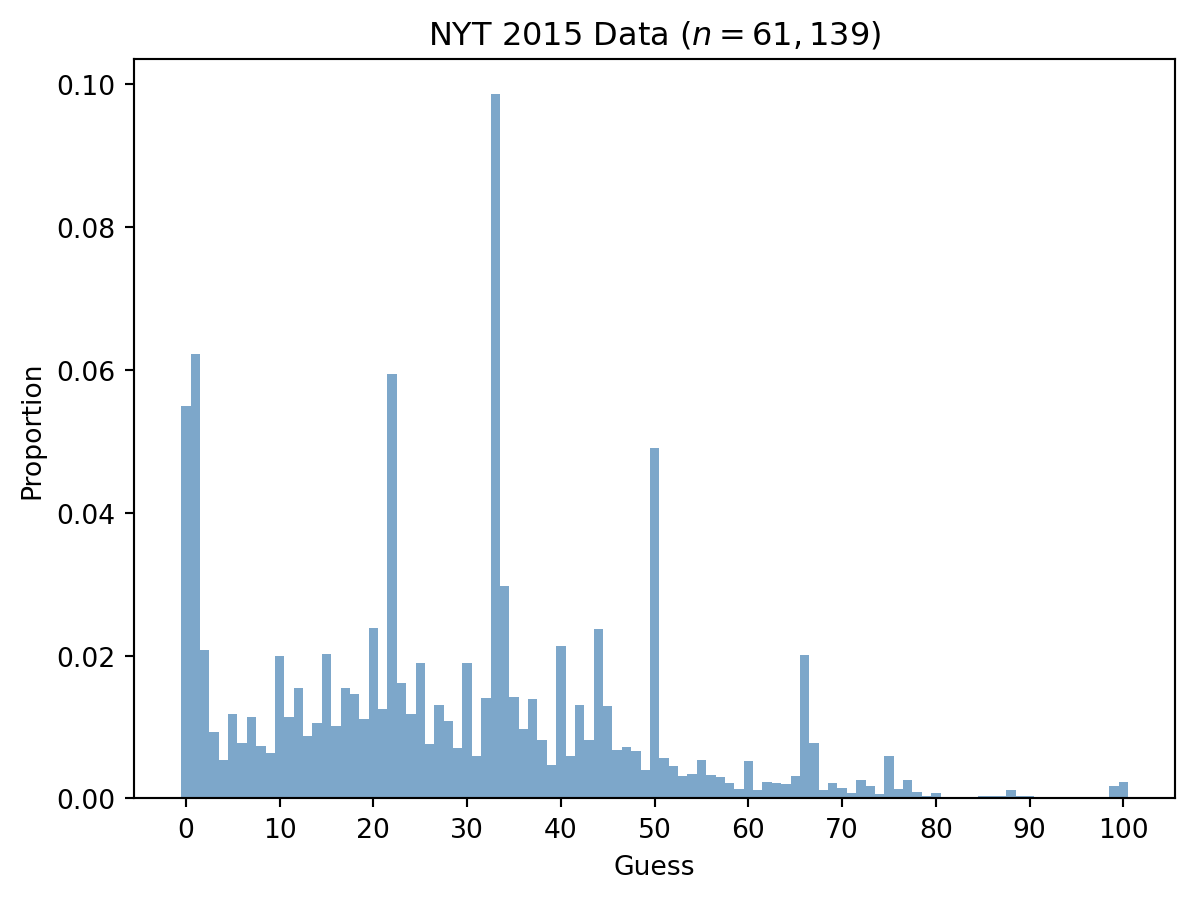

The data shows several peaks: one around 33 (level 0 reasoning: 2/3 of 50), one around 22 (level 1: 2/3 of 33), and smaller peaks at lower values corresponding to higher levels of reasoning. There are also anomalous peaks at 50 and 66 that don’t fit any level of reasoning—presumably from readers who misunderstood the game.

Mixture model

Our model assumes that each reader reasons at a single level k. But different readers may reason at different levels. We can model this heterogeneity with a mixture: a weighted combination of level-specific distributions.

Let \pi_k be the fraction of readers thinking at level k, and let P_k(n \mid \beta) be the probability that a level-k reader guesses n (given inverse temperature \beta). The mixture model predicts:

P(n) = \sum_{k=0}^{K-1} \pi_k \cdot P_k(n \mid \beta)

We’ll fit both the level weights \pi and the inverse temperature \beta to minimize the squared error between model predictions and the empirical distribution.

def predict_mixture(log_weights, beta):
    """Compute mixture model predictions across all levels."""
    weights = jnp.exp(log_weights)  ### softmax parameterization for weights
    predictions = sum(
        w * reader_choice_k_soft(k=k, beta=beta)
        for k, w in enumerate(weights)
    )
    return predictions / jnp.sum(predictions)

def loss_fn(log_weights, beta):
    """Mean squared error between model and data."""
    pred = predict_mixture(log_weights, beta)
    return jnp.sum((nyt - pred) ** 2)

We use gradient descent to find the best-fitting parameters.

### Initialize parameters
log_weights = jnp.zeros(10)  ### 10 levels (0-9), uniform initial weights
beta = jnp.array(1.0)        ### initial inverse temperature

### Gradient descent
learning_rate = 10.0
for t in range(201):
    loss, (grad_w, grad_b) = jax.value_and_grad(loss_fn, argnums=(0, 1))(log_weights, beta)
    log_weights = log_weights - learning_rate * grad_w
    beta = beta - learning_rate * grad_b
    if t % 50 == 0:
        print(f"Step {t:>3}: loss = {loss:.6f}")

print(f"\nFit β = {beta:.2f}")

Step   0: loss = 0.041870
Step  50: loss = 0.015312
Step 100: loss = 0.014831
Step 150: loss = 0.014521
Step 200: loss = 0.014318

Fit β = 0.66

Let’s visualize how well the fitted model captures the data.

pred = predict_mixture(log_weights, beta)

fig, ax = plt.subplots(figsize=(10, 5))
_ = ax.bar(N, nyt, color='steelblue', alpha=0.5, label='NYT data')
_ = ax.plot(N, pred, 'o-', color='darkorange', linewidth=2, markersize=3, label='Mixture model')
_ = ax.set_xticks(N[::10])
_ = ax.set_xlabel('Guess')
_ = ax.set_ylabel('Frequency')
_ = ax.set_title('Model fit to NYT 2015 data')
_ = ax.legend()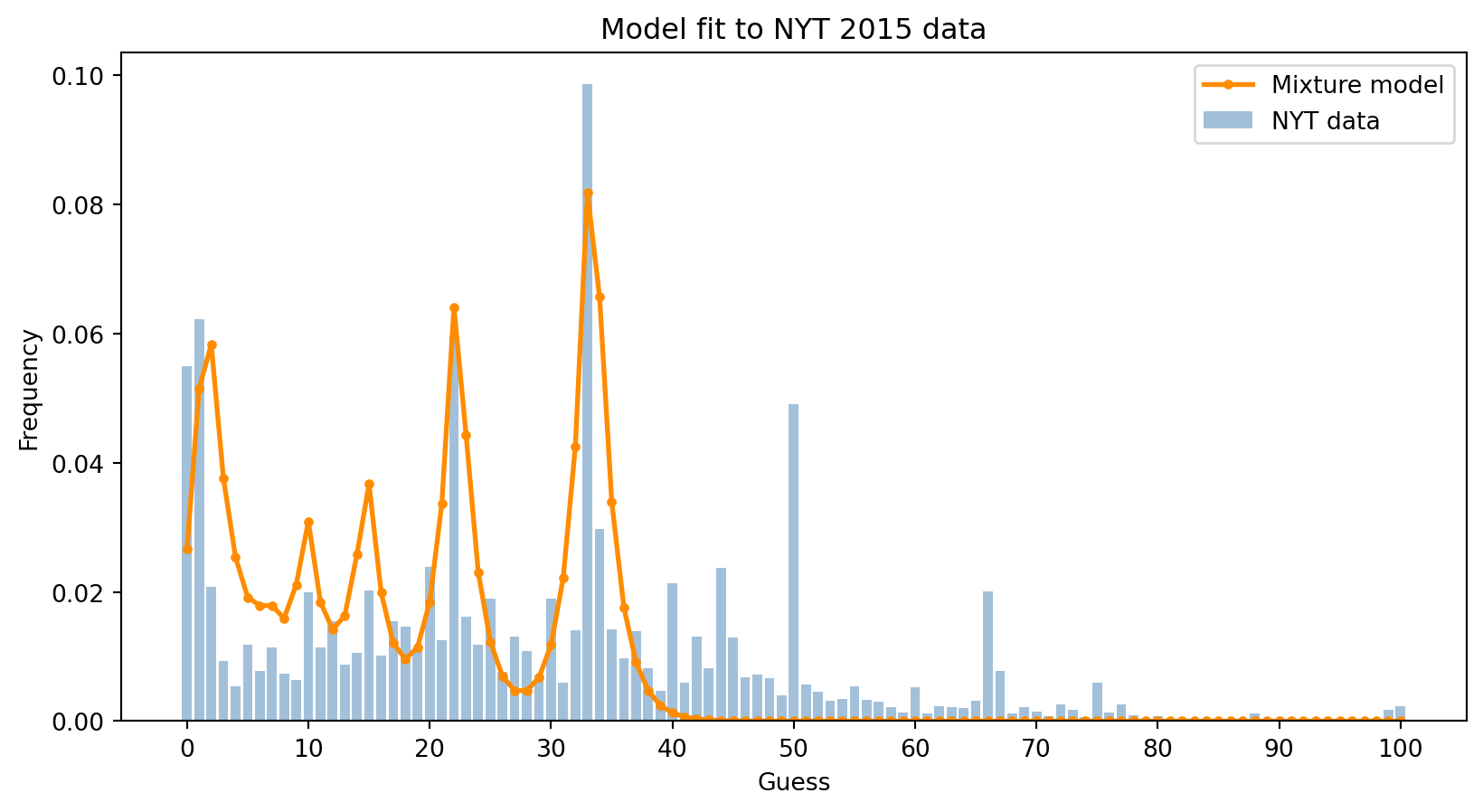

The mixture model captures the main structure of the data: the peaks at 33, 22, 15, and lower values corresponding to different levels of recursive reasoning. However, it cannot explain the peaks at 50 and 66—these guesses don’t correspond to any level of game-theoretic reasoning and likely reflect readers who didn’t fully understand the rules.

Inferred distribution of reasoning levels

By examining the fitted weights, we can estimate what fraction of NYT readers were thinking at each level.

weights = jnp.exp(log_weights)
weights = weights / jnp.sum(weights)

fig, ax = plt.subplots()
_ = ax.bar(range(len(weights)), weights, color='steelblue')
_ = ax.set_xticks(range(len(weights)))
_ = ax.set_xlabel('Level k')
_ = ax.set_ylabel('Fraction of readers')
_ = ax.set_title('Inferred distribution of reasoning levels')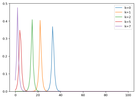

The distribution suggests that most NYT readers engaged in relatively shallow reasoning (levels 0-2), with smaller fractions reasoning at higher levels. This is consistent with prior findings in behavioral economics: most people do not reason all the way to the Nash equilibrium, even in games with clear strategic structure.

Exercises

In what ways does the reader_choice_k_soft model capture the empirical NYT data well? What cognitive processes seem poorly captured by the model?
Extend the reader_choice_k_soft model to capture some aspect of the data that the model captures poorly.
Build a memo model where:
- Agent A chooses a number from -3 to 9 (inclusive) with uniform probability.
- Agent B thinks that Agent C chooses either 7 or 8 with equal probability.
- Agent C thinks that Agent D chooses a number from 1 to 3 (inclusive) with uniform probability.
- Agent C chooses a number from 0 to 9 (inclusive) with uniform probability.
All choices should take the form chooses(v in V, wpp=...) and use the same sample space, V = jnp.arange(-3, 9 + 1).

Have the model return:

A. The expected value of Agent A’s choice.

B. Agent B’s expectation of Agent C’s choice.

C. Agent C’s expectation of Agent D’s choice.

For A, B & C, you can submit the same model with different return statements, or return multiple values jointly, like so:
```
@memo
def f():
    reader1: chooses(a in N, wpp=1)
    reader2: chooses(b in N, wpp=1)
    reader3: chooses(c in N, wpp=1)
    return E[reader1.a]
    return E[reader2.b] / 2
    return E[reader3.c] / 3

resf = f()
print(f"First  index of resf : E[reader1.a]    = {resf[0]:0.4f}")
print(f"Second index of resf : E[reader2.b]/2  = {resf[1]:0.4f}")
print(f"Third  index of resf : E[reader3.c]/3  = {resf[2]:0.4f}")
```
```
First  index of resf : E[reader1.a]    = 50.0003
Second index of resf : E[reader2.b]/2  = 25.0002
Third  index of resf : E[reader3.c]/3  = 16.6666
```

Render env

%reset -f
import sys
import platform
import importlib.metadata

print("Python:", sys.version)
print("Platform:", platform.system(), platform.release())
print("Processor:", platform.processor())
print("Machine:", platform.machine())

print("\nPackages:")
for name, version in sorted(
    ((dist.metadata["Name"], dist.version) for dist in importlib.metadata.distributions()),
    key=lambda x: x[0].lower()  # Sort case-insensitively
):
    print(f"{name}=={version}")

Python: 3.14.2 (main, Dec  5 2025, 21:11:58) [Clang 21.1.4 ]
Platform: Darwin 24.6.0
Processor: arm
Machine: arm64

Packages:
altair==6.0.0
annotated-types==0.7.0
anyio==4.12.1
anywidget==0.9.21
appnope==0.1.4
argon2-cffi==25.1.0
argon2-cffi-bindings==25.1.0
arrow==1.4.0
astroid==4.0.3
asttokens==3.0.1
async-lru==2.0.5
attrs==25.4.0
babel==2.17.0
beautifulsoup4==4.14.3
bleach==6.3.0
certifi==2026.1.4
cffi==2.0.0
cfgv==3.5.0
charset-normalizer==3.4.4
click==8.3.1
comm==0.2.3
contourpy==1.3.3
cycler==0.12.1
debugpy==1.8.19
decorator==5.2.1
defusedxml==0.7.1
dill==0.4.0
distlib==0.4.0
docutils==0.22.4
executing==2.2.1
fastjsonschema==2.21.2
filelock==3.20.3
fonttools==4.61.1
fqdn==1.5.1
h11==0.16.0
httpcore==1.0.9
httpx==0.28.1
identify==2.6.16
idna==3.11
importlib_metadata==8.7.1
ipykernel==7.1.0
ipython==9.9.0
ipython_pygments_lexers==1.1.1
ipywidgets==8.1.8
isoduration==20.11.0
isort==7.0.0
itsdangerous==2.2.0
jax==0.8.2
jaxlib==0.8.2
jedi==0.19.2
Jinja2==3.1.6
joblib==1.5.3
json5==0.13.0
jsonpointer==3.0.0
jsonschema==4.26.0
jsonschema-specifications==2025.9.1
jupyter-cache==1.0.1
jupyter-events==0.12.0
jupyter-lsp==2.3.0
jupyter_client==8.8.0
jupyter_core==5.9.1
jupyter_server==2.17.0
jupyter_server_terminals==0.5.4
jupyterlab==4.5.2
jupyterlab_pygments==0.3.0
jupyterlab_server==2.28.0
jupyterlab_widgets==3.0.16
kiwisolver==1.4.9
lark==1.3.1
marimo==0.19.4
Markdown==3.10
MarkupSafe==3.0.3
matplotlib==3.10.8
matplotlib-inline==0.2.1
mccabe==0.7.0
memo-lang==1.2.9
mistune==3.2.0
ml_dtypes==0.5.4
msgspec==0.20.0
narwhals==2.15.0
nbclient==0.10.4
nbconvert==7.16.6
nbformat==5.10.4
nest-asyncio==1.6.0
networkx==3.6.1
nodeenv==1.10.0
notebook_shim==0.2.4
numpy==2.4.1
numpy-typing-compat==20251206.2.4
opt_einsum==3.4.0
optype==0.15.0
packaging==25.0
pandas==2.3.3
pandas-stubs==2.3.3.260113
pandocfilters==1.5.1
parso==0.8.5
pexpect==4.9.0
pillow==12.1.0
platformdirs==4.5.1
plotly==5.24.1
pre_commit==4.5.1
prometheus_client==0.24.1
prompt_toolkit==3.0.52
psutil==7.2.1
psygnal==0.15.1
ptyprocess==0.7.0
pure_eval==0.2.3
pycparser==2.23
pydantic==2.12.5
pydantic_core==2.41.5
Pygments==2.19.2
pygraphviz==1.14
pylint==4.0.4
pymdown-extensions==10.20
pyparsing==3.3.1
python-dateutil==2.9.0.post0
python-dotenv==1.2.1
python-json-logger==4.0.0
pytz==2025.2
PyYAML==6.0.3
pyzmq==27.1.0
referencing==0.37.0
requests==2.32.5
rfc3339-validator==0.1.4
rfc3986-validator==0.1.1
rfc3987-syntax==1.1.0
rpds-py==0.30.0
ruff==0.14.13
scikit-learn==1.8.0
scipy==1.17.0
scipy-stubs==1.17.0.1
seaborn==0.13.2
Send2Trash==2.1.0
setuptools==80.9.0
six==1.17.0
soupsieve==2.8.1
SQLAlchemy==2.0.45
stack-data==0.6.3
starlette==0.51.0
tabulate==0.9.0
tenacity==9.1.2
terminado==0.18.1
threadpoolctl==3.6.0
tinycss2==1.4.0
toml==0.10.2
tomlkit==0.14.0
tornado==6.5.4
tqdm==4.67.1
traitlets==5.14.3
types-pytz==2025.2.0.20251108
typing-inspection==0.4.2
typing_extensions==4.15.0
tzdata==2025.3
uri-template==1.3.0
urllib3==2.6.3
uvicorn==0.40.0
virtualenv==20.36.1
wcwidth==0.2.14
webcolors==25.10.0
webencodings==0.5.1
websocket-client==1.9.0
websockets==16.0
widgetsnbextension==4.0.15
xarray==2025.12.0
zipp==3.23.0

References

Luce, Robert Duncan. (1959). Individual choice behavior: A theoretical analysis. Wiley. https://books.google.com?id=a80DAQAAIAAJ

Nagel, Rosemarie. (1995). Unraveling in Guessing Games: An Experimental Study. The American Economic Review, 85(5), 1313–1326. http://www.jstor.org/stable/2950991

Footnotes

You might be wondering why n, which is bound to the reader’s mental model of the population’s collective mind is not also bracketed. In fact it is—the dot notation is just a convenient shorthand; this return statement could also be written reader[ E[population[n]] ].↩︎
NB you could equivalently write this as an \mathrm{argmax} by maximizing the negative absolute error: to_maximize = -abs( (2/3)*E[population.n] - n ).↩︎

Modeling agentic choice

Parametric priors

Query variables

Details and examples

Indexing output

Empty axes

Identity of query variables

Using a @memo as a submodel

Encapsulation in mental frames

Choice based on mental simulation

Recursive reasoning

Approximately rational choice

Softmax

Interactive exploration of the softmax function

Interactive exploration softmax parameter in the game

Model fitting

Mixture model

Inferred distribution of reasoning levels

Exercises

References

Footnotes

Using a `@memo` as a submodel