import jax
import jax.numpy as jnp
from memo import memo
from memo import domain as product
from enum import IntEnum
from matplotlib import pyplot as pltConditional dependence
Patterns of inference as evidence changes
In the previous chapter, we saw that two variables can be statistically dependent—knowing one changes what we should believe about the other. But dependence is not a fixed property. It can appear or disappear depending on what else we know. Two variables that are dependent can become independent once we learn the value of a third variable (screening off), and two variables that are independent can become dependent once we learn something else (explaining away). These shifts are determined by the causal structure connecting the variables. This chapter introduces the basic causal motifs—fork, pipe, collider, and descendent—and shows how each one governs the way dependence changes with evidence.
Causal motifs
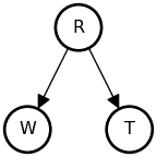
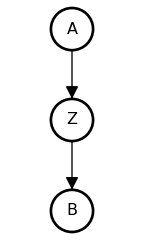
The Fork
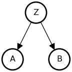
Z is a “common cause” of A and B
• A and B are associated: {A \not\perp B}
• Share a common cause Z
• Once stratified by Z (conditioned on Z), no association: {A \perp B \mid Z}
• A and B are associated: {A \not\perp B}
• Share a common cause Z
• Once stratified by Z (conditioned on Z), no association: {A \perp B \mid Z}
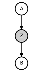
The Pipe

Z is a “mediator” of A and B
• A and B are associated: {A \not\perp B}
• Influence of A on B transmitted through Z
• Once stratified by Z, no association: {A \perp B \mid Z}
• A and B are associated: {A \not\perp B}
• Influence of A on B transmitted through Z
• Once stratified by Z, no association: {A \perp B \mid Z}
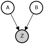
The Collider (Immorality)
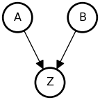
Z is a “collider” of A and B
• A and B are not associated (no shared causes): {A \perp B}
• A and B both influence Z
• Once stratified by Z, A and B are associated: {A \not\perp B \mid Z}
• A and B are not associated (no shared causes): {A \perp B}
• A and B both influence Z
• Once stratified by Z, A and B are associated: {A \not\perp B \mid Z}
The Descendent
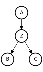
C is a “descendent”
• A and B are causally associated through Z: {A \not\perp B}
• C carries information about Z
• Conditioning on C partially screens off A from B, since C provides indirect evidence about Z
• A and B are causally associated through Z: {A \not\perp B}
• C carries information about Z
• Conditioning on C partially screens off A from B, since C provides indirect evidence about Z
Conditional independence
Recall the definition of (in)dependence. We define conditional (in)dependence in effectively the same way, just conditioning everything on a new random variable, Z. So whereas (marginal) independence is defined as { A \perp B \iff P(A, \, B) = P(A) \; P(B) }, conditional independence is defined as:
A \perp B \mid Z \iff P(A, \, B \mid Z) = P(A \mid Z) \; P(B \mid Z) \\ \text{where}~~~ P(Z) > 0 \\ \forall~ (a, b, z) \in \{ \mathcal{A} \times \mathcal{B} \times \mathcal{Z} \}
And in the same way as we saw for marginal independence,
A \perp B \mid Z ~~\iff~~ P(A \mid B, \, Z) = P(A \mid Z)
Exercise: Show that, if {A \perp B \mid Z}, then {P(B \mid A, \, Z) = P(B \mid Z)}. Hint: Follow the chain rule.
NoteSolution
In general (regardless of dependence),
P(A, \, B \mid Z) = P(A \mid Z) \; P(B \mid A, \, Z) \\ \forall~ (a, b, z) \in \{ \mathcal{A} \times \mathcal{B} \times \mathcal{Z} \} ~~~\text{where}~~~ P(A, \, Z) > 0
If {A \perp B \mid Z}, then {P(A, \, B \mid Z) = P(A \mid Z) \; P(B \mid Z)}.
In which case,
P(A \mid Z) \; P(B \mid Z) = P(A \mid Z) \; P(B \mid A, \, Z)
and {P(B \mid Z) = P(B \mid A, \, Z)}.
From A Priori Dependence to Conditional Dependence
The relationships between causal structure and statistical dependence become particularly interesting and subtle when we look at the effects of additional observations or assumptions. Events that are statistically dependent a priori may become independent when we condition on some observation; this is called screening off. Also, events that are statistically independent a priori may become dependent when we condition on observations; this is known as explaining away. The dynamics of screening off and explaining away are extremely important for understanding patterns of inference—reasoning and learning—in probabilistic models.
Screening off
Screening off refers to a pattern of statistical inference that is quite common in both scientific and intuitive reasoning. If the statistical dependence between two events A and B is only indirect, mediated strictly by one or more other events Z, then conditioning on (observing) Z should render A and B statistically independent. This can occur if A and B are connected by one or more causal chains, and all such chains run through the set of events Z, or if Z comprises all of the common causes of A and B.
Fork
For instance, let’s look at a common cause example (a “fork”). Here, A and B are associated ({A \not\perp B}). We can determine this by observing that { P(A \mid B{=}\mathtt{true}) \neq P(A \mid B{=}\mathtt{false}) }.

class A(IntEnum):
    FALSE = 0
    TRUE = 1

class B(IntEnum):
    FALSE = 0
    TRUE = 1

class Z(IntEnum):
    FALSE = 0
    TRUE = 1

@memo
def fork[_a: A, _b: B]():
    agent: knows(_a, _b)
    agent: thinks[
        friend: knows(_a, _b),
        friend: chooses(z in Z, wpp=1),
        friend: chooses(a in A, wpp=(
            1 if z == {Z.TRUE}
            else (0.9 if a == {A.TRUE} else 0.1))),
        friend: chooses(b in B, wpp=(
            (
                0.1 if b == {B.TRUE} else 0.9
            ) if z == {Z.TRUE}
            else (0.4 if b == {B.TRUE} else 0.6))),
    ]

    ### this observes statement is just here to
    ### make it easier to inspect the results
    agent: observes [friend.b] is _b

    return agent[Pr[friend.a == _a]]

res = fork(print_table=True, return_aux=True, return_xarray=True)

resx = res.aux.xarray
print("\n")
for a in A:
    for b in B:
        a_, b_ = a.name, b.name
        print(f"P(A={a_} | B={b_}) = {resx.loc[a_, b_].item():0.4f}")
    print("---")
+-------+-------+----------------------+
| _a: A | _b: B | fork |
+-------+-------+----------------------+
| FALSE | FALSE | 0.3399999737739563 |
| FALSE | TRUE | 0.18000000715255737 |
| TRUE | FALSE | 0.6599999666213989 |
| TRUE | TRUE | 0.8199999928474426 |
+-------+-------+----------------------+
P(A=FALSE | B=FALSE) = 0.3400
P(A=FALSE | B=TRUE) = 0.1800
---
P(A=TRUE | B=FALSE) = 0.6600
P(A=TRUE | B=TRUE) = 0.8200
---
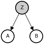
NoteConditioning on B
Note: The DAG above shows the model {P(A, B, Z)}. However, the @memo (fork) is conditioned on B — this done purely because it’s easier to visually inspect if { P(A \mid B) = P(A \mid \neg B) = P(A) } than it is to inspect if { P(A, B) = P(A) \; P(B) }.
The conceptually important part is what happens when the model is conditioned on Z, so while I am conditioning the model on B, I’m not shading the B node in the DAG.
We could, of course, run the model that’s actually shown in the DAG by removing the agent: observes [friend.b] is _b line, and then check if { P(A, B) = P(A) \; P(B) } (see the Without extra conditional details for a demonstration).
TipWithout extra conditional
In the joint model, { P(A, B) \neq P(A) \; P(B) }.
@memo
def fork_joint[_a: A, _b: B]():
    agent: knows(_a, _b)
    agent: thinks[
        friend: knows(_a, _b),
        friend: chooses(z in Z, wpp=1),
        friend: chooses(a in A, wpp=(
            1 if z == {Z.TRUE}
            else (0.9 if a == {A.TRUE} else 0.1))),
        friend: chooses(b in B, wpp=(
            (
                0.1 if b == {B.TRUE} else 0.9
            ) if z == {Z.TRUE}
            else (0.4 if b == {B.TRUE} else 0.6))),
    ]

    ### without observes statement
    # agent: observes [friend.b] is _b

    return agent[Pr[friend.a == _a, friend.b == _b]]

res = fork_joint(print_table=True, return_aux=True, return_xarray=True)

resx = res.aux.xarray
print("\nCompare:")
for a in A:
    for b in B:
        a_, b_ = a.name, b.name
        print("\n")
        print(f"P(A={a_}, B={b_}) = {resx.loc[a_, b_].item():0.4f}")
        print(f"P(A={a_}) P(B={b_}) = {resx.loc[a_, :].sum().item() * resx.loc[:, b_].sum().item():0.4f}")
+-------+-------+----------------------+
| _a: A | _b: B | fork_joint |
+-------+-------+----------------------+
| FALSE | FALSE | 0.2549999952316284 |
| FALSE | TRUE | 0.04500000178813934 |
| TRUE | FALSE | 0.4950000047683716 |
| TRUE | TRUE | 0.20499999821186066 |
+-------+-------+----------------------+
Compare:
P(A=FALSE, B=FALSE) = 0.2550
P(A=FALSE) P(B=FALSE) = 0.2250
P(A=FALSE, B=TRUE) = 0.0450
P(A=FALSE) P(B=TRUE) = 0.0750
P(A=TRUE, B=FALSE) = 0.4950
P(A=TRUE) P(B=FALSE) = 0.5250
P(A=TRUE, B=TRUE) = 0.2050
P(A=TRUE) P(B=TRUE) = 0.1750But once stratified by Z (i.e., conditioned on Z), { P(A, B \mid Z) } is always equal to { P(A \mid Z) \; P(B \mid Z) }.
@memo
def fork_joint__z[_z: Z, _a: A, _b: B]():
    agent: knows(_a, _b, _z)
    agent: thinks[
        friend: knows(_a, _b),
        friend: chooses(z in Z, wpp=1),
        friend: chooses(a in A, wpp=(
            1 if z == {Z.TRUE}
            else (0.9 if a == {A.TRUE} else 0.1))),
        friend: chooses(b in B, wpp=(
            (
                0.1 if b == {B.TRUE} else 0.9
            ) if z == {Z.TRUE}
            else (0.4 if b == {B.TRUE} else 0.6))),
    ]

    agent: observes [friend.z] is _z

    ### without observes statement
    # agent: observes [friend.b] is _b

    return agent[Pr[friend.a == _a, friend.b == _b]]

res = fork_joint__z(print_table=True, return_aux=True, return_xarray=True)

resx = res.aux.xarray

print("\nCompare:")
for z in Z:
    for a in A:
        for b in B:
            z_, a_, b_ = z.name, a.name, b.name
            print("\n")
            print(f"  P(A={a_}, B={b_} | Z={z_}) = {resx.loc[z_, a_, b_].item():0.4f}")
            print(f"  P(A={a_} | Z={z_}) P(B={b_} | Z={z_}) = {resx.loc[z_, a_, :].sum().item() * resx.loc[z_, :, b_].sum().item():0.4f}")
+-------+-------+-------+----------------------+
| _z: Z | _a: A | _b: B | fork_joint__z |
+-------+-------+-------+----------------------+
| FALSE | FALSE | FALSE | 0.06000000238418579 |
| FALSE | FALSE | TRUE | 0.04000000283122063 |
| FALSE | TRUE | FALSE | 0.5400000214576721 |
| FALSE | TRUE | TRUE | 0.35999998450279236 |
| TRUE | FALSE | FALSE | 0.44999998807907104 |
| TRUE | FALSE | TRUE | 0.05000000074505806 |
| TRUE | TRUE | FALSE | 0.44999998807907104 |
| TRUE | TRUE | TRUE | 0.05000000074505806 |
+-------+-------+-------+----------------------+
Compare:
P(A=FALSE, B=FALSE | Z=FALSE) = 0.0600
P(A=FALSE | Z=FALSE) P(B=FALSE | Z=FALSE) = 0.0600
P(A=FALSE, B=TRUE | Z=FALSE) = 0.0400
P(A=FALSE | Z=FALSE) P(B=TRUE | Z=FALSE) = 0.0400
P(A=TRUE, B=FALSE | Z=FALSE) = 0.5400
P(A=TRUE | Z=FALSE) P(B=FALSE | Z=FALSE) = 0.5400
P(A=TRUE, B=TRUE | Z=FALSE) = 0.3600
P(A=TRUE | Z=FALSE) P(B=TRUE | Z=FALSE) = 0.3600
P(A=FALSE, B=FALSE | Z=TRUE) = 0.4500
P(A=FALSE | Z=TRUE) P(B=FALSE | Z=TRUE) = 0.4500
P(A=FALSE, B=TRUE | Z=TRUE) = 0.0500
P(A=FALSE | Z=TRUE) P(B=TRUE | Z=TRUE) = 0.0500
P(A=TRUE, B=FALSE | Z=TRUE) = 0.4500
P(A=TRUE | Z=TRUE) P(B=FALSE | Z=TRUE) = 0.4500
P(A=TRUE, B=TRUE | Z=TRUE) = 0.0500
P(A=TRUE | Z=TRUE) P(B=TRUE | Z=TRUE) = 0.0500Now let’s assume that we already know the value of Z:
@memo
def fork__z[_z: Z, _a: A, _b: B]():
    agent: knows(_a, _b, _z)
    agent: thinks[
        friend: knows(_a, _b),
        friend: chooses(z in Z, wpp=1),
        friend: chooses(a in A, wpp=(
            1 if z == {Z.TRUE}
            else (0.9 if a == {A.TRUE} else 0.1))),
        friend: chooses(b in B, wpp=(
            (
                0.1 if b == {B.TRUE} else 0.9
            ) if z == {Z.TRUE}
            else (0.4 if b == {B.TRUE} else 0.6))),
    ]

    agent: observes [friend.z] is _z

    ### this observes statement is just here to
    ### make it easier to inspect the results
    agent: observes [friend.b] is _b

    return agent[Pr[friend.a == _a]]

res = fork__z(print_table=True, return_aux=True, return_xarray=True)
+-------+-------+-------+----------------------+
| _z: Z | _a: A | _b: B | fork__z |
+-------+-------+-------+----------------------+
| FALSE | FALSE | FALSE | 0.10000000149011612 |
| FALSE | FALSE | TRUE | 0.10000001639127731 |
| FALSE | TRUE | FALSE | 0.8999999761581421 |
| FALSE | TRUE | TRUE | 0.9000000357627869 |
| TRUE | FALSE | FALSE | 0.5 |
| TRUE | FALSE | TRUE | 0.5 |
| TRUE | TRUE | FALSE | 0.5 |
| TRUE | TRUE | TRUE | 0.5 |
+-------+-------+-------+----------------------+We see that {A \perp B \mid Z}. While A and B are marginally dependent, they are conditionally independent given knowledge of Z.
E.g.
print(f"if A and B are conditionally independent given Z, then...")
resx = res.aux.xarray
for z in Z:
    for a in A:
        print("\nThese should be the same:")
        for b in B:
            z_, a_, b_ = z.name, a.name, b.name
            print(f"  P(A={a_} | B={b_}, Z={z_}) = {resx.loc[z_, a_, b_].item():0.4f}")
if A and B are conditionally independent given Z, then...
These should be the same:
P(A=FALSE | B=FALSE, Z=FALSE) = 0.1000
P(A=FALSE | B=TRUE, Z=FALSE) = 0.1000
These should be the same:
P(A=TRUE | B=FALSE, Z=FALSE) = 0.9000
P(A=TRUE | B=TRUE, Z=FALSE) = 0.9000
These should be the same:
P(A=FALSE | B=FALSE, Z=TRUE) = 0.5000
P(A=FALSE | B=TRUE, Z=TRUE) = 0.5000
These should be the same:
P(A=TRUE | B=FALSE, Z=TRUE) = 0.5000
P(A=TRUE | B=TRUE, Z=TRUE) = 0.5000Continuous Fork
Joint Probability Heatmap
### Import
def lobf(x, y):
    import numpy as np
    return (np.unique(x), np.poly1d(jnp.polyfit(x, y, 1))(np.unique(x)))

def jointprob_facetgrid(P, support_dim0=None, support_dim1=None, origin=True, corr=True, cmap="BuPu", dim0: dict | None = None, dim1: dict | None = None, **kwargs):
    import seaborn as sns
    import numpy as np
    import matplotlib.pyplot as plt

    if support_dim0 is None:
        support_dim0 = np.arange(P.shape[0])
    if support_dim1 is None:
        support_dim1 = np.arange(P.shape[1])
    if isinstance(dim0, dict) and "support" in dim0:
        support_dim0 = dim0["support"]
    if isinstance(dim1, dict) and "support" in dim1:
        support_dim1 = dim1["support"]

    label_dim0 = "dim 0"
    label_dim1 = "dim 1"
    lim_dim0 = None
    lim_dim1 = None

    label_dim0 = kwargs.get("label_dim0", label_dim0)
    label_dim1 = kwargs.get("label_dim1", label_dim1)

    lim_dim0 = kwargs.get("lim_dim0", lim_dim0)
    lim_dim1 = kwargs.get("lim_dim0", lim_dim1)

    title = kwargs.get("title", None)

    if isinstance(dim0, dict):
        label_dim0 = dim0.get("label", label_dim0)
        lim_dim0 = dim0.get("lim", lim_dim0)
    if isinstance(dim1, dict):
        label_dim1 = dim1.get("label", label_dim1)
        lim_dim1 = dim0.get("lim", lim_dim1)

    assert len(P.shape) == 2
    assert len(support_dim0.shape) == 1
    assert len(support_dim1.shape) == 1

    # Create the grid for the joint plot with shared axes
    g = sns.JointGrid(ratio=8, height=4)
    g.ax_marg_x.sharex(g.ax_joint)
    g.ax_marg_y.sharey(g.ax_joint)

    # Plot the main density with contours
    contour = g.ax_joint.contourf(support_dim0, support_dim1, P.T, levels=20, cmap=cmap, norm="linear", )
    g.ax_joint.contour(support_dim0, support_dim1, P.T, levels=10, colors="white", alpha=0.3, linewidths=0.5)

    xlim = g.ax_joint.get_xlim()
    ylim = g.ax_joint.get_ylim()

    if origin:
        _ = g.ax_joint.axhline(0, color="white", linewidth=0.5, alpha=0.3)
        _ = g.ax_joint.axvline(0, color="white", linewidth=0.5, alpha=0.3)

    # Plot marginal distributions with aligned axes
    g.ax_marg_x.set_facecolor('#f0f0f0')
    g.ax_marg_y.set_facecolor('#f0f0f0')
    g.ax_marg_x.fill_between(support_dim0, P.sum(axis=1), alpha=0.3)
    g.ax_marg_y.fill_betweenx(support_dim1, P.sum(axis=0), alpha=0.3)

    if corr:
        # Calculate expected values
        A, B = np.meshgrid(support_dim0, support_dim1)
        E_a = np.sum(A * P.T) / np.sum(P)
        E_b = np.sum(B * P.T) / np.sum(P)

        # Calculate covariance
        cov_ab = np.sum((A - E_a) * (B - E_b) * P.T) / np.sum(P)
        var_a = np.sum((A - E_a)**2 * P.T) / np.sum(P)
        var_b = np.sum((B - E_b)**2 * P.T) / np.sum(P)

        # Calculate correlation
        correlation = cov_ab / np.sqrt(var_a * var_b)

        # Calculate line of best fit
        slope = cov_ab / var_a
        intercept = E_b - slope * E_a

        # Plot line of best fit
        line_x = np.array([support_dim0[0], support_dim0[-1]])
        line_y = slope * line_x + intercept
        g.ax_joint.plot(line_x, line_y, "w--", linewidth=1, label=f'r = {correlation:.2f}')
        # g.ax_joint.legend()

    g.ax_joint.set_xlim(xlim)
    g.ax_joint.set_ylim(ylim)

    E_d0 = np.sum(support_dim0 * P.sum(axis=1))
    E_d1 = np.sum(support_dim1 * P.sum(axis=0))
    g.ax_marg_x.scatter(E_d0, 0.0, color="red", s=15, marker="v", label="E[d0]")
    g.ax_marg_y.scatter(0.0, E_d1, color="red", s=15, marker="<", label="E[d1]")


    g.ax_marg_y.tick_params(labelleft=False, direction='in')

    # Remove ticks from marginal plots
    # g.ax_marg_x.tick_params(labelbottom=False)
    # g.ax_marg_y.tick_params(labelleft=False)

    g.ax_marg_x.tick_params(labelbottom=False, direction='in')
    g.ax_marg_y.tick_params(labelleft=False, direction='in')

    if label_dim0 is not None:
        _ = g.ax_joint.set_xlabel(label_dim0)
    if label_dim0 is not None:
        _ = g.ax_joint.set_ylabel(label_dim1)

    if lim_dim0 is not None:
        _ = g.ax_joint.set_xlim(lim_dim0)
    if lim_dim1 is not None:
        _ = g.ax_joint.set_ylim(lim_dim1)

    if title:
        _ = g.figure.suptitle(title, y=1.03)

    return g
from jax.scipy.stats.norm import pdf as normpdf
normpdfjit = jax.jit(normpdf)
W = jnp.linspace(-3, 3, 11)
T = jnp.linspace(-3, 3, 11)
R = jnp.arange(2)
@memo
def viz_fork_joint[_w: W, _t: T]():
agent: knows(_w, _t)
agent: thinks[
friend: chooses(r in R, wpp=1),
friend: chooses(w in W, wpp=normpdfjit(w, 2*r-1, 0.5)),
friend: chooses(t in T, wpp=normpdfjit(t, 2*r-1, 0.5)),
]
return agent[Pr[friend.w == _w, friend.t == _t]]
fig = jointprob_facetgrid(viz_fork_joint(), W, T,
label_dim0="W", label_dim1="T", title=r"$P(W, T)$", cmap="inferno")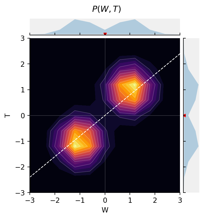
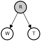
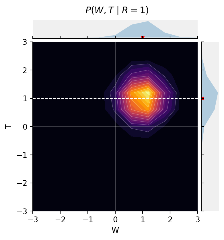
But, when we stratify by R, now {W \perp T \mid R}.
from jax.scipy.stats.norm import pdf as normpdf

normpdfjit = jax.jit(normpdf)

W = jnp.linspace(-3, 3, 11)
T = jnp.linspace(-3, 3, 11)
R = jnp.arange(2)

@memo
def viz_fork_stratified[_w: W, _t: T, _r: R]():
    agent: knows(_w, _t)
    agent: thinks[
        friend: chooses(r in R, wpp=1),
        friend: chooses(w in W, wpp=normpdfjit(w, 2*r-1, 0.5)),
        friend: chooses(t in T, wpp=normpdfjit(t, 2*r-1, 0.5)),
    ]
    agent: observes [friend.r] is _r
    return agent[Pr[friend.w == _w, friend.t == _t]]

res = viz_fork_stratified()

fig = jointprob_facetgrid(
    res[:, :, 0],
    W,
    T,
    label_dim0="W",
    label_dim1="T",
    title=r"$P(W, T \mid R{=}0)$",
    cmap="inferno")
fig = jointprob_facetgrid(
    res[:, :, 1],
    W,
    T,
    label_dim0="W",
    label_dim1="T",
    title=r"$P(W, T \mid R{=}1)$",
    cmap="inferno")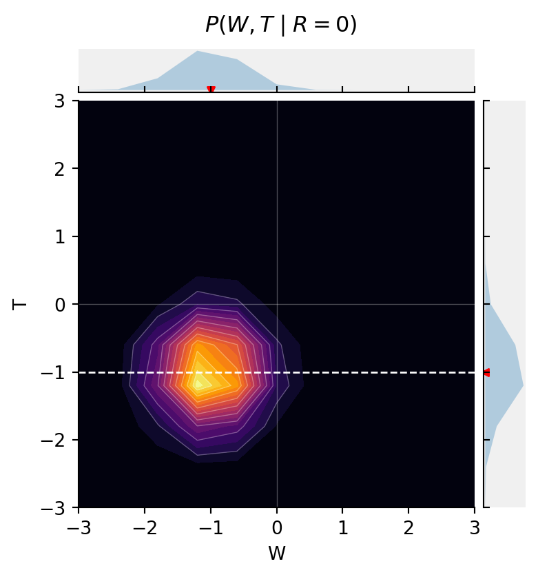
Pipe
Screening off is a purely statistical phenomenon. For example, consider the causal chain model, where A directly causes Z, which in turn directly causes B (Z is a “mediator”).
@memo
def pipe[_a: A, _b: B]():
    agent: knows(_a, _b)
    agent: thinks[
        friend: knows(_a, _b),
        friend: chooses(a in A, wpp=1),
        friend: chooses(z in Z, wpp=(
            1 if a == {A.TRUE}
            else (0.9 if z == {Z.TRUE} else 0.1))),
        friend: chooses(b in B, wpp=(
            (
                0.1 if b == {B.TRUE} else 0.9
            ) if z == {Z.TRUE}
            else (0.4 if b == {B.TRUE} else 0.6))),
    ]
    ### this observes statement is just here to
    ### make it easier to inspect the results
    agent: observes [friend.b] is _b
    return agent[Pr[friend.a == _a]]

_ = pipe(print_table=True)
+-------+-------+---------------------+
| _a: A | _b: B | pipe |
+-------+-------+---------------------+
| FALSE | FALSE | 0.5370370149612427 |
| FALSE | TRUE | 0.3421052396297455 |
| TRUE | FALSE | 0.4629629850387573 |
| TRUE | TRUE | 0.6578946709632874 |
+-------+-------+---------------------+We can observe that A and B are associated.
But observing Z, the event that mediates an indirect causal relation between A and B, renders A and B independent. A and B are still causally dependent in our model, it is just our beliefs about the states of A and B that become conditionally independent.
@memo
def pipe[_z: Z, _a: A, _b: B]():
    agent: knows(_a, _b, _z)
    agent: thinks[
        friend: knows(_a, _b),
        friend: chooses(a in A, wpp=1),
        friend: chooses(z in Z, wpp=(
            1 if a == {A.TRUE}
            else (0.9 if z == {Z.TRUE} else 0.1))),
        friend: chooses(b in B, wpp=(
            (
                0.1 if b == {B.TRUE} else 0.9
            ) if z == {Z.TRUE}
            else (0.4 if b == {B.TRUE} else 0.6))),
    ]

    agent: observes [friend.z] is _z

    ### this observes statement is just here to
    ### make it easier to inspect the results
    agent: observes [friend.b] is _b

    return agent[Pr[friend.a == _a]]

_ = pipe(print_table=True)
+-------+-------+-------+---------------------+
| _z: Z | _a: A | _b: B | pipe |
+-------+-------+-------+---------------------+
| FALSE | FALSE | FALSE | 0.1666666567325592 |
| FALSE | FALSE | TRUE | 0.1666666865348816 |
| FALSE | TRUE | FALSE | 0.8333333134651184 |
| FALSE | TRUE | TRUE | 0.8333333134651184 |
| TRUE | FALSE | FALSE | 0.6428571343421936 |
| TRUE | FALSE | TRUE | 0.6428571343421936 |
| TRUE | TRUE | FALSE | 0.3571428656578064 |
| TRUE | TRUE | TRUE | 0.3571428954601288 |
+-------+-------+-------+---------------------+Explaining away
“Explaining away” (Pearl, 2014) refers to a complementary pattern of statistical inference which is somewhat more subtle than screening off. If two events A and B are causally independent (and hence, a priori, statistically independent), but they are both causes of one or more other events Z, then conditioning on (observing) Z can render A and B statistically dependent. Here is an example where A and B have a common effect (they collide on Z).
@memo
def collider_marginal[_a: A, _b: B]():
    agent: knows(_a, _b)
    agent: thinks[
        friend: knows(_a, _b),
        friend: chooses(a in A, wpp=1),
        friend: chooses(b in B, wpp=1),
        friend: chooses(z in Z, wpp=(
            (
                0.9 if z == {Z.TRUE} else 0.1
            ) if (a == {A.TRUE} or b == {B.TRUE})
            else (0.2 if z == {Z.TRUE} else 0.8))),
    ]

    ### this observes statement is just here to
    ### make it easier to inspect the results
    agent: observes [friend.b] is _b

    return agent[Pr[friend.a == _a]]

_ = collider_marginal(print_table=True)
+-------+-------+--------------------+
| _a: A | _b: B | collider_marginal |
+-------+-------+--------------------+
| FALSE | FALSE | 0.5 |
| FALSE | TRUE | 0.5 |
| TRUE | FALSE | 0.5 |
| TRUE | TRUE | 0.5 |
+-------+-------+--------------------+Without conditioning on Z, A and B are independent: { P(A \mid B{=}\mathtt{true}) = P(A \mid B{=}\mathtt{false}) }.
But once we condition on Z:
@memo
def collider[_z: Z, _a: A, _b: B]():
    agent: knows(_a, _b, _z)
    agent: thinks[
        friend: knows(_a, _b),
        friend: chooses(a in A, wpp=1),
        friend: chooses(b in B, wpp=1),
        friend: chooses(z in Z, wpp=(
            (
                0.9 if z == {Z.TRUE} else 0.1
            ) if (a == {A.TRUE} or b == {B.TRUE})
            else (0.2 if z == {Z.TRUE} else 0.8))),
    ]

    agent: observes [friend.z] is _z

    ### this observes statement is just here to
    ### make it easier to inspect the results
    agent: observes [friend.b] is _b

    return agent[Pr[friend.a == _a]]

_ = collider(print_table=True)
+-------+-------+-------+---------------------+
| _z: Z | _a: A | _b: B | collider |
+-------+-------+-------+---------------------+
| FALSE | FALSE | FALSE | 0.8888888359069824 |
| FALSE | FALSE | TRUE | 0.5 |
| FALSE | TRUE | FALSE | 0.1111111044883728 |
| FALSE | TRUE | TRUE | 0.5 |
| TRUE | FALSE | FALSE | 0.1818181872367859 |
| TRUE | FALSE | TRUE | 0.5 |
| TRUE | TRUE | FALSE | 0.8181818127632141 |
| TRUE | TRUE | TRUE | 0.5 |
+-------+-------+-------+---------------------+now { P(A \mid B{=}\mathtt{true}, Z) \neq P(A \mid B{=}\mathtt{false}, Z) }. Learning about B gives us information about A because both A and B are potential explanations for Z.
As with screening off, we only induce statistical dependence from learning about Z, not causal dependence: when we observe Z, A and B remain causally independent in our model of the world; it is our beliefs about A and B that become statistically dependent.
The most typical pattern of explaining away we see in causal reasoning is a kind of anti-correlation: the probabilities of two possible causes for the same effect increase when the effect is observed, but they are conditionally anti-correlated, so that observing additional evidence in favor of one cause should lower our degree of belief in the other cause. (This pattern is where the term explaining away comes from.) However, the coupling induced by conditioning on common effects depends on the nature of the interaction between the causes, it is not always an anti-correlation. Explaining away takes the form of an anti-correlation when the causes interact in a roughly disjunctive or additive form: the effect tends to happen if any cause happens; or the effect happens if the sum of some continuous influences exceeds a threshold. The following simple mathematical examples show this and other patterns.
The model below defines two independent variables X and Y both of which are used to define the value of our data. Suppose we condition on observing the sum of two integers drawn uniformly from 0 to 9:
from jax.scipy.stats.norm import pdf as normpdf

normpdfjit = jax.jit(normpdf)

X = jnp.arange(10)
Y = jnp.arange(10)

@memo
def f[_x: X, _y: Y]():
    agent: knows(_x, _y)
    agent: thinks[
        selection: chooses(x in X, wpp=1),
        selection: chooses(y in Y, wpp=1),
    ]
    agent: observes_that[ selection.x + selection.y == 9 ]

    return agent[Pr[selection.x == _x, selection.y == _y]]

g = jointprob_facetgrid(
    f(),
    X,
    Y,
    label_dim0="X",
    label_dim1="Y",
    title=r"$P(X, Y \mid X+Y=9)$",
    cmap="inferno")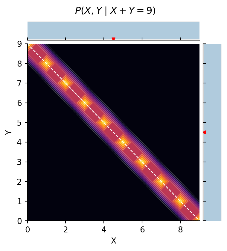
This gives perfect anti-correlation in conditional inferences for X and Y. But suppose we instead condition on observing that X and Y are equal:
@memo
def ff[_x: X, _y: Y]():
    agent: knows(_x, _y)
    agent: thinks[
        selection: chooses(x in X, wpp=1),
        selection: chooses(y in Y, wpp=1),
    ]
    agent: observes_that[ selection.x == selection.y ]

    return agent[Pr[selection.x == _x, selection.y == _y]]

g = jointprob_facetgrid(
    ff(),
    X,
    Y,
    label_dim0="X",
    label_dim1="Y",
    title=r"$P(X, Y \mid X=Y)$",
    cmap="inferno")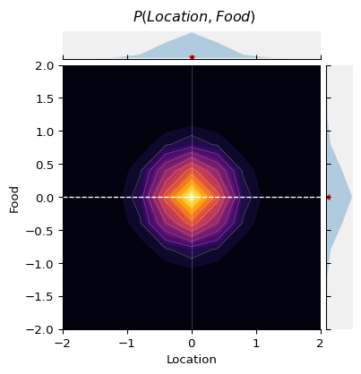
Now, of course, X and Y go from being independent a priori to being perfectly correlated in the conditional distribution. Try out these other conditions to see other possible patterns of conditional dependence for a priori independent functions:
selection.x - selection.y < 2
selection.x + selection.y >= 9 and selection.x + selection.y <= 11
abs(selection.x - selection.y) == 3
(selection.x - selection.y) % 10 == 3
selection.x % 2 == selection.y % 2
selection.x % 5 == selection.y % 5
selection.x % 2 == selection.y % 3
@memo
def fff[_x: X, _y: Y]():
agent: knows(_x, _y)
agent: thinks[
selection: chooses(x in X, wpp=1),
selection: chooses(y in Y, wpp=1),
]
agent: observes_that[ abs(selection.x - selection.y) == 3 ]
return agent[Pr[selection.x == _x, selection.y == _y]]
g = jointprob_facetgrid(
fff(),
X,
Y,
label_dim0="X",
label_dim1="Y",
title=r"$P(X, Y \mid |X-Y|=3)$",
cmap="inferno")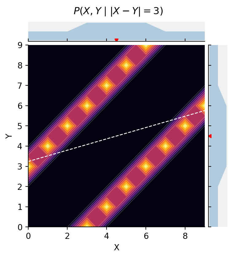
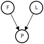
Collider - selection and survivorship bias
Restaurants
This model looks at the effect of conditioning on a collider.
It is not uncommon that restaurants with amazing food require some effort to get to, while convenient locations are filled with mediocre restaurants that somehow stay in business.
A restaurant’s popularity depends both on its food and its location. Restaurants with exceptional food can thrive in out-of-the-way locations because people will make the extra effort to visit them. Restaurants in prime locations (think busy downtowns and tourist hotspots) can get away with serving subpar food because they get plenty of foot traffic or it’s hard for people to go elsewhere (think airports, music festivals, and rural college campuses).
The model represents this by measuring both food quality and location on a scale where 0 is “average,” positive numbers are “better than average,” and negative numbers are “worse than average.” Popularity is modeled as the combination of food and location. The popularity_value function sums the food and location values for a given restaurant. A restaurant is more likely to be popular if the food is good and if it’s easy to get to. This function also represents the idea that popularity isn’t perfectly determined by food and location alone. There are other factors that influence a restaurant’s popularity (things like ambiance, live music and staff). These other factors are modeled as isomorphic Gaussian noise centered on \text{food} + \text{location}:
\begin{align*} \text{food} ~\sim& ~~\mathcal{N}(\mu{=}0, \sigma_{\text{food}}) \\ \text{location} ~\sim& ~~\mathcal{N}(\mu{=}0, \sigma_{\text{location}}) \\ \text{popularity} ~\sim& ~~\mathcal{N}(\mu{=}\text{food}+\text{location}, \sigma_{\text{popularity}}) \end{align*}
from jax.scipy.stats.norm import pdf as normpdf

normpdfjit = jax.jit(normpdf)

Food = jnp.linspace(-2, 2, 11)
Location = jnp.linspace(-2, 2, 11)
Popularity = product(
    food=len(Food),
    loc=len(Location),
)

@jax.jit
def popularity_value(p):
    y_food = Popularity.food(p)
    y_loc = Popularity.loc(p)
    return y_food + y_loc

@jax.jit
def popularity_pdf(p, f, l):
    return normpdf(popularity_value(p), f + l, 0.4)

@memo
def critic_joint[_f: Food, _l: Location](cutoff=1):
    critic: knows(_f, _l)
    critic: thinks[
        restaurant: knows(_f, _l),
        restaurant: chooses(f in Food, wpp=normpdfjit(f, 0, 0.4)),
        restaurant: chooses(l in Location, wpp=normpdfjit(l, 0, 0.4)),
        clientele: knows(restaurant.f, restaurant.l),
        clientele: chooses(p in Popularity, wpp=popularity_pdf(p, restaurant.f, restaurant.l))
    ]

    return critic[Pr[restaurant.f == _f, restaurant.l == _l]]

g = jointprob_facetgrid(
    critic_joint(),
    Food,
    Location,
    label_dim0="Location",
    label_dim1="Food",
    title=r"$P(Location,Food)$",
    cmap="inferno")
This plot shows the probability density of { P(\text{location}, \text{food}) }, as well as the marginal distributions { P(\text{location}) } above and { P(\text{food}) } to the right. The dashed red line is the correlation between Location and Food.
As you can see, there is no a priori association between the quality of food and the location.
However, in order for a restaurant to survive, it must attract a certain number of clientele.
In the model below, we introduce a selection criterion. Restaurants that do not exceed the minimum popularity cutoff go out of business.
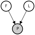
Below, we condition the model on {\text{popularity} > 1}. Restaurants more popular than the cutoff survive while the others go out of business. We depict this conditioning by shading the “popularity” node in the DAG.
@memo
def critic_posterior[_f: Food, _l: Location](cutoff=1):
    critic: knows(_f, _l)
    critic: thinks[
        restaurant: knows(_f, _l),
        restaurant: chooses(f in Food, wpp=normpdfjit(f, 0, 0.4)),
        restaurant: chooses(l in Location, wpp=normpdfjit(l, 0, 0.4)),

        clientele: knows(restaurant.f, restaurant.l),
        clientele: chooses(p in Popularity, wpp=popularity_pdf(p, restaurant.f, restaurant.l))
    ]

    critic: observes_that[ popularity_value(clientele.p) > cutoff ]

    return critic[Pr[restaurant.f == _f, restaurant.l == _l]]

cutoff_ = 1
g = jointprob_facetgrid(
    critic_posterior(cutoff=cutoff_),
    Food,
    Location,
    label_dim0="Location",
    label_dim1="Food",
    title=fr"$P(Location,Food \mid popularity > {cutoff_})$",
    cmap="inferno")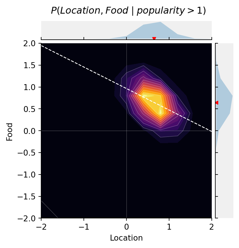
The selection criterion induces a negative correlation between Location and Food. Try changing the cutoff value and see what happens to the correlation. The more stringent the selection, the stronger the correlation.
Really good restaurants can survive in bad locations because they’re worth the effort of getting to, and terrible restaurants can survive in Hanover because it’s hard for the population to go elsewhere.
This simple example illustrates a very common phenomenon in causal inference: selection on a variable changes associations between the variable’s causal antecedents. In this case, conditioning on the collider P induced statistical dependence between the causally independent variables, F and L.
Statistical intuition for explaining away
To build intuition for why conditioning on a common effect induces dependence between the causes, consider the simplest possible collider: two independent fair coins A and B, with a common effect Z = A \lor B (“at least one is true”).
The prior joint distribution {P(A, B)} is uniform—each cell has probability \frac{1}{4}:
\boxed{\begin{array}{r|c|c|l} & \neg B & B & \\ \hline A & \tfrac{1}{4} & \tfrac{1}{4} & \colorbox{#dbeafe}{$P(A) = \tfrac{1}{2}$} \\ \hline \neg A & \tfrac{1}{4} & \tfrac{1}{4} & \colorbox{#dbeafe}{$P(\neg A) = \tfrac{1}{2}$} \\ \hline & \colorbox{#dbeafe}{$P(\neg B) = \tfrac{1}{2}$} & \colorbox{#dbeafe}{$P(B) = \tfrac{1}{2}$} & \end{array}}
When we condition on Z{=}\mathtt{true} (i.e., A \lor B), we eliminate the one cell where both \neg A and \neg B. The three surviving cells are equally probable:
\begin{array}{r|cc|l} & \neg B & B & \\ \hline A & \tfrac{1}{3} & \tfrac{1}{3} & P(A \mid Z) = \tfrac{2}{3} \\[6pt] \neg A & \colorbox{#e8e8e8}{$\cancel{\;\tfrac{1}{4}\;}$} & \tfrac{1}{3} & P(\neg A \mid Z) = \tfrac{1}{3} \\ \hline & P(\neg B \mid Z) = \tfrac{1}{3} & P(B \mid Z) = \tfrac{2}{3} & \end{array}
Marginalizing: P(A \mid Z) = \frac{2}{3} and P(B \mid Z) = \frac{2}{3}. Both went up from their prior of \frac{1}{2}—but the ratio is still 1{:}1. Observing only Z tells us nothing about whether A or B is more likely than the other.
Now suppose we additionally learn that B is true. This restricts us to the right column of the table—only two cells survive:
\begin{array}{r|c|l} & B & \\ \hline A & \tfrac{1}{2} & P(A \mid B, Z) = \tfrac{1}{2} \\[6pt] \neg A & \tfrac{1}{2} & P(\neg A \mid B, Z) = \tfrac{1}{2} \\ \hline & P(B \mid B, Z) = 1 & \end{array}
P(A \mid B, Z) = \frac{1}{2}, down from \frac{2}{3}. Learning that B is true has explained away some of the evidence for A. The ratio P(A) / P(B), which was 1{:}1 after observing only Z, has shifted to \frac{1}{2} (that is, \frac{1}{2} versus 1).
The cell-counting makes this transparent. Among the three cells consistent with Z, two have B but only one of those two also has A. Once we learn we are in the B column, A is true in only half the remaining possibilities—whereas before, A was true in two of three.
This is the discrete version of the same phenomenon shown in the continuous examples below and in the restaurant model: conditioning on a common effect (here, A \lor B; there, popularity exceeding a threshold) creates a negative dependence between the causes. The more one cause accounts for the effect, the less the other needs to.
Summary
The key patterns of conditional dependence are determined by causal structure:
| Motif | Structure | Marginal | Conditional on Z |
|---|---|---|---|
| Fork (common cause) | A \leftarrow Z \rightarrow B | A \not\perp B | A \perp B \mid Z |
| Pipe (mediator) | A \rightarrow Z \rightarrow B | A \not\perp B | A \perp B \mid Z |
| Collider (common effect) | A \rightarrow Z \leftarrow B | A \perp B | A \not\perp B \mid Z |
- Screening off: Conditioning on a common cause or mediator renders its effects conditionally independent. The intuition is that Z carries all the information that A and B share, so once Z is known, A provides no additional information about B.
- Explaining away: Conditioning on a common effect induces dependence between its causes. Learning that Z occurred, together with information about one cause, changes what we should believe about the other cause.
Exercises
Consider a medical scenario: a disease (D) causes both a fever (F) and a rash (R). Draw the DAG. Are F and R marginally dependent or independent? What happens to the dependence between F and R if you learn the patient’s disease status?
Now consider: both a cold (C) and allergies (A) can cause a runny nose (N). Draw the DAG. Are C and A marginally dependent or independent? What happens when you learn the patient has a runny nose?
A university admits students based on a combination of test scores (T) and interview performance (I). Among the general applicant population, T and I are independent. What pattern of dependence would you expect between T and I among admitted students? Which causal motif does this correspond to?
NoteRender env
%reset -f
import sys
import platform
import importlib.metadata

print("Python:", sys.version)
print("Platform:", platform.system(), platform.release())
print("Processor:", platform.processor())
print("Machine:", platform.machine())

print("\nPackages:")
for name, version in sorted(
    ((dist.metadata["Name"], dist.version) for dist in importlib.metadata.distributions()),
    key=lambda x: x[0].lower()  # Sort case-insensitively
):
    print(f"{name}=={version}")
Python: 3.14.3 (main, Feb 4 2026, 01:51:49) [Clang 21.1.4 ]
Platform: Darwin 24.6.0
Processor: arm
Machine: arm64
Packages:
altair==6.0.0
annotated-types==0.7.0
anyio==4.12.1
anywidget==0.9.21
appnope==0.1.4
argon2-cffi==25.1.0
argon2-cffi-bindings==25.1.0
arrow==1.4.0
astroid==4.0.4
asttokens==3.0.1
async-lru==2.1.0
attrs==25.4.0
babel==2.18.0
beautifulsoup4==4.14.3
bleach==6.3.0
certifi==2026.1.4
cffi==2.0.0
cfgv==3.5.0
charset-normalizer==3.4.4
click==8.3.1
colour-science==0.4.7
comm==0.2.3
contourpy==1.3.3
cycler==0.12.1
debugpy==1.8.20
decorator==5.2.1
defusedxml==0.7.1
dill==0.4.1
distlib==0.4.0
distro==1.9.0
docutils==0.22.4
executing==2.2.1
fastjsonschema==2.21.2
filelock==3.20.3
fonttools==4.61.1
fqdn==1.5.1
h11==0.16.0
httpcore==1.0.9
httpx==0.28.1
identify==2.6.16
idna==3.11
importlib_metadata==8.7.1
ipykernel==7.2.0
ipython==9.10.0
ipython_pygments_lexers==1.1.1
ipywidgets==8.1.8
isoduration==20.11.0
isort==7.0.0
itsdangerous==2.2.0
jax==0.9.0.1
jaxlib==0.9.0.1
jedi==0.19.2
Jinja2==3.1.6
jiter==0.13.0
joblib==1.5.3
json5==0.13.0
jsonpointer==3.0.0
jsonschema==4.26.0
jsonschema-specifications==2025.9.1
jupyter-cache==1.0.1
jupyter-events==0.12.0
jupyter-lsp==2.3.0
jupyter_client==8.8.0
jupyter_core==5.9.1
jupyter_server==2.17.0
jupyter_server_terminals==0.5.4
jupyterlab==4.5.3
jupyterlab_pygments==0.3.0
jupyterlab_server==2.28.0
jupyterlab_widgets==3.0.16
kiwisolver==1.4.9
lark==1.3.1
marimo==0.19.9
Markdown==3.10.1
MarkupSafe==3.0.3
matplotlib==3.10.8
matplotlib-inline==0.2.1
mccabe==0.7.0
memo-lang==1.2.9
mistune==3.2.0
ml_dtypes==0.5.4
msgspec==0.20.0
narwhals==2.16.0
nbclient==0.10.4
nbconvert==7.17.0
nbformat==5.10.4
nest-asyncio==1.6.0
networkx==3.6.1
nodeenv==1.10.0
notebook_shim==0.2.4
numpy==2.4.2
numpy-typing-compat==20251206.2.4
openai==2.17.0
opt_einsum==3.4.0
optype==0.15.0
packaging==26.0
pandas==3.0.0
pandas-stubs==3.0.0.260204
pandocfilters==1.5.1
parso==0.8.5
patsy==1.0.2
pexpect==4.9.0
pillow==12.1.0
platformdirs==4.5.1
plotly==5.24.1
pre_commit==4.5.1
prometheus_client==0.24.1
prompt_toolkit==3.0.52
psutil==7.2.2
psygnal==0.15.1
ptyprocess==0.7.0
pure_eval==0.2.3
pycparser==3.0
pydantic==2.12.5
pydantic_core==2.41.5
Pygments==2.19.2
pygraphviz==1.14
pylint==4.0.4
pymdown-extensions==10.20.1
pyparsing==3.3.2
python-dateutil==2.9.0.post0
python-dotenv==1.2.1
python-json-logger==4.0.0
PyYAML==6.0.3
pyzmq==27.1.0
referencing==0.37.0
requests==2.32.5
rfc3339-validator==0.1.4
rfc3986-validator==0.1.1
rfc3987-syntax==1.1.0
rpds-py==0.30.0
ruff==0.15.0
scikit-learn==1.8.0
scipy==1.17.0
scipy-stubs==1.17.0.2
seaborn==0.13.2
Send2Trash==2.1.0
setuptools==81.0.0
six==1.17.0
sniffio==1.3.1
soupsieve==2.8.3
SQLAlchemy==2.0.46
stack-data==0.6.3
starlette==0.52.1
statsmodels==0.14.6
tabulate==0.9.0
tenacity==9.1.4
terminado==0.18.1
threadpoolctl==3.6.0
tinycss2==1.4.0
toml==0.10.2
tomlkit==0.14.0
tornado==6.5.4
tqdm==4.67.3
traitlets==5.14.3
typing-inspection==0.4.2
typing_extensions==4.15.0
tzdata==2025.3
uri-template==1.3.0
urllib3==2.6.3
uvicorn==0.40.0
virtualenv==20.36.1
wcwidth==0.6.0
webcolors==25.10.0
webencodings==0.5.1
websocket-client==1.9.0
websockets==16.0
widgetsnbextension==4.0.15
xarray==2026.1.0
zipp==3.23.0References
Pearl, Judea. (2014). Probabilistic Reasoning in Intelligent Systems: Networks of Plausible Inference (1. Aufl). Elsevier Reference Monographs.