Factorization

Solution to the in-class exercise

The paper we read, Baker et al. (2017), gives the following posterior proportionality in Eq. (1):

\Pr(B_0, B_1, D, P, S | A) \propto \Pr(A | B_1, D) \times \Pr(B_1 | P, B_0) \times \Pr(P | S) \times \Pr(B_0, D, S) \tag{1}

From Bayes’ rule we know that

\Pr(\mathcal{H} | \mathcal{D}) = \frac{\Pr(\mathcal{H}) \times \Pr(\mathcal{D} | \mathcal{H})}{\Pr(\mathcal{D})} = \frac{\Pr(\mathcal{H}, \mathcal{D})}{\Pr(\mathcal{D})}

such that { \Pr(\mathcal{H} | \mathcal{D}) \propto \Pr(\mathcal{H}, \mathcal{D}) }.

Thus, Equation 1 can be reexpressed

\Pr(B_0, B_1, D, P, S | A) \propto \Pr(B_0, B_1, D, P, S, A)

Can we derive the factorization of the joint probability given in Equation 1? That is,

\Pr(B_0, B_1, D, P, S, A) = \Pr(A | B_1, D) \times \Pr(B_1 | P, B_0) \times \Pr(P | S) \times \Pr(B_0, D, S) \tag{2}

Let’s start by applying the chain rule:

\begin{align*} \Pr(B_0, B_1, D, &P, S, A) = \\ &\Pr(B_0) \times \Pr(B_1 | B_0) \times \Pr(D | B_0, B_1) \times \Pr(P | B_0, B_1, D) \\ &\quad\quad\times \Pr(S | B_0, B_1, D, P) \times \Pr(A | B_0, B_1, D, P, S) \end{align*}

Making eleminations based on the conditional dependencies given by the causal structure:

\begin{align*} &\Pr(B_0) \times \Pr(B_1 | B_0) \times \Pr(D | \sout{B_0}, \sout{B_1}) \times \Pr(P | B_0, B_1, \sout{D}) \\ &\quad\quad \times \Pr(S | \sout{B_0}, \sout{B_1}, \sout{D}, P) \times \Pr(A | \sout{B_0}, B_1, D, \sout{P}, \sout{S}) \\ &= \Pr(B_0) \times \Pr(B_1 | B_0) \times \Pr(D) \times \Pr(P | B_0, B_1) \times \Pr(S | P) \times \Pr(A | B_1, D) \end{align*} \tag{3}

Notice that we can’t make any additional eliminations from { \Pr(P | B_0, B_1) } because { P \not\perp B_0 \mid B_1 }. While P and B_0 are statistically independent a priori, conditioning on B_1 induces statistical dependence between P and B_0 (recall the collider bias and the other causal motifs).

Similarly, while S is causally independent of P (causal influce flows in the direction of arrows), information flows both directions so S and P are statistically dependent {( S \not\perp P )}. Knowing something about P gives you information about S and vice versa (recall the definition of statistical dependence).

The equality we’re trying to derive (i.e. Equation 2) is

\Pr(B_0, B_1, D, P, S, A) = \Pr(A | B_1, D) \times \biggl[ \Pr(B_1 | P, B_0) \times \Pr(P | S) \times \Pr(S) \biggr] \times \Pr(B_0) \times \Pr(D) \tag{4}

And after our factorization and eliminations (i.e. Equation 3) we’ve arrived at

\Pr(B_0, B_1, D, P, S, A) = \Pr(A | B_1, D) \times \biggl[ \Pr(B_1 | B_0) \times \Pr(P | B_0, B_1) \times \Pr(S | P) \biggr] \times \Pr(B_0) \times \Pr(D) \tag{5}

The brackets show the terms that differ between Equation 4 and Equation 5. But we can refactor these terms to show that they are equivalent.

First,

\begin{align*} \Pr(B_1 | B_0) \times \Pr(P | B_0, B_1) = \Pr(B_1, P | B_0) &= \Pr(P | B_0) \times \Pr(B_1 | B_0, P) \\ &= \Pr(P | \sout{B_0}) \times \Pr(B_1 | B_0, P) ~~~\text{since}~~ P \perp B_0 \\ &= \Pr(P) \times \Pr(B_1 | B_0, P) \end{align*}

Meaning that

\biggl[ \Pr(B_1 | B_0) \times \Pr(P | B_0, B_1) \times \Pr(S | P) \biggr] = \Pr(P) \times \Pr(B_1 | B_0, P) \times \Pr(S | P)

And similarly,

\Pr(P) \times \Pr(S | P) = \Pr(S, P) = \Pr(S) \times \Pr(P | S)

Thus, the bracketed terms from the original factorization (Equation 4) and in our factorization (Equation 5) are equivalent:

\biggl[ \Pr(B_1 | B_0) \times \Pr(P | B_0, B_1) \times \Pr(S | P) \biggr] = \Pr(B_1 | B_0, P) \times \Pr(S) \times \Pr(P | S)

And plugging this expression of the bracketed term back into our factorization, we arrive at Equation 2.

\begin{align*} \Pr(B_0, B_1, D, P, S, A) &= \Pr(B_0) \times \Pr(D) \times \Pr(A | B_1, D) \times \biggl[ \Pr(B_1 | B_0, P) \times \Pr(S) \times \Pr(P | S) \biggr] \\ &= \Pr(A | B_1, D) \times \Pr(B_1 | P, B_0) \times \Pr(P | S) \times \Pr(S) \times \Pr(D) \times \Pr(B_0) \\ &= \Pr(A | B_1, D) \times \Pr(B_1 | P, B_0) \times \Pr(P | S) \times \Pr(B_0, D, S) \end{align*}

A different factorization

Now let’s try applying the chain rule in a different order.

\begin{align*} &\Pr(B_0, B_1, D, P, S, A) \\ &\quad= \Pr(B_0) \times \Pr(D | B_0) \times \Pr(S | B_0, D) \times \Pr(P | B_0, D, S ) \times \Pr(B_1 | B_0, D, S, P) \times \Pr(A | B_0, D, S, P, B_1) \\ % &\quad=\Pr(B_0) \times \Pr(D | \sout{B_0}) \times \Pr(S | \sout{B_0}, \sout{D}) \times \Pr(P | \sout{B_0}, \sout{D}, S) \times \Pr(B_1 | B_0, \sout{D}, \sout{S}, P) \times \Pr(A | \sout{B_0}, D, \sout{S}, \sout{P}, B_1) \\ % &\quad=\Pr(B_0) \times \Pr(D) \times \Pr(S) \times \Pr(P | S) \times \Pr(B_1 | B_0, P) \times \Pr(A | D, B_1) \\ % &\quad=\Pr(A | D, B_1) \times \Pr(B_1 | B_0, P) \times \Pr(P | S) \times Pr(B_0, D, S) \end{align*}

Wow, that was easier. Why didn’t we just do that to start? Because we didn’t know what order of variables to use.

Exercises

  1. Based on the posterior given in Equation 1, what is the prior, likelihood and marginal evidence?

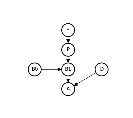
  2. In Equation 3, we used the conditional independencies of the causal graph to expresses { \Pr(S | B_0, B_1, D, P) } as { \Pr(S | P) }. Explain why the causal graph permits the elimination of B_0, B_1, and D, and not P. For instance, we condition on B_1, which is a collider of S and B_1. Why can we still eliminate B_1?

  3. We have shown that there are multiple (potentially very many) factorizations of a joint distribution that are probabilistically equivalent. E.g. in the worked example, \begin{align*} \Pr(B_0, B_1, &D, P, S, A) \\=&\\ \Pr(A | B_1, D) \times \Pr(B_1 | P, B_0) &\times \Pr(P | S) \times\Pr(S, B_0, D) \\=&\\ \Pr(A | B_1, D) \times \Pr(B_1 | B_0) \times& \Pr(P | B_0, B_1) \times \Pr(S | P) \times \Pr(B_0) \times \Pr(D) \end{align*}

    Why did these authors chose the former factorization rather than the latter, or any of the myriad other factorizations that are mathematically equivalent? Why bother factorizing at all? Why not just use the joint probability { \Pr(B_0, B_1, D, P, S, A) }?


%reset -f
import sys
import platform
import importlib.metadata

print("Python:", sys.version)
print("Platform:", platform.system(), platform.release())
print("Processor:", platform.processor())
print("Machine:", platform.machine())

print("\nPackages:")
for name, version in sorted(
    ((dist.metadata["Name"], dist.version) for dist in importlib.metadata.distributions()),
    key=lambda x: x[0].lower()  # Sort case-insensitively
):
    print(f"{name}=={version}")
Python: 3.13.2 (main, Feb  5 2025, 18:58:04) [Clang 19.1.6 ]
Platform: Darwin 23.6.0
Processor: arm
Machine: arm64

Packages:
annotated-types==0.7.0
anyio==4.9.0
appnope==0.1.4
argon2-cffi==23.1.0
argon2-cffi-bindings==21.2.0
arrow==1.3.0
astroid==3.3.9
asttokens==3.0.0
async-lru==2.0.5
attrs==25.3.0
babel==2.17.0
beautifulsoup4==4.13.3
bleach==6.2.0
certifi==2025.1.31
cffi==1.17.1
cfgv==3.4.0
charset-normalizer==3.4.1
click==8.1.8
comm==0.2.2
contourpy==1.3.1
cycler==0.12.1
debugpy==1.8.13
decorator==5.2.1
defusedxml==0.7.1
dill==0.3.9
distlib==0.3.9
executing==2.2.0
fastjsonschema==2.21.1
filelock==3.18.0
fonttools==4.56.0
fqdn==1.5.1
h11==0.14.0
httpcore==1.0.7
httpx==0.28.1
identify==2.6.9
idna==3.10
importlib_metadata==8.6.1
ipykernel==6.29.5
ipython==9.0.2
ipython_pygments_lexers==1.1.1
ipywidgets==8.1.5
isoduration==20.11.0
isort==6.0.1
jax==0.5.3
jaxlib==0.5.3
jedi==0.19.2
Jinja2==3.1.6
joblib==1.4.2
json5==0.10.0
jsonpointer==3.0.0
jsonschema==4.23.0
jsonschema-specifications==2024.10.1
jupyter-cache==1.0.1
jupyter-events==0.12.0
jupyter-lsp==2.2.5
jupyter_client==8.6.3
jupyter_core==5.7.2
jupyter_server==2.15.0
jupyter_server_terminals==0.5.3
jupyterlab==4.3.6
jupyterlab_pygments==0.3.0
jupyterlab_server==2.27.3
jupyterlab_widgets==3.0.13
kiwisolver==1.4.8
MarkupSafe==3.0.2
matplotlib==3.10.1
matplotlib-inline==0.1.7
mccabe==0.7.0
memo-lang==1.1.2
mistune==3.1.3
ml_dtypes==0.5.1
nbclient==0.10.2
nbconvert==7.16.6
nbformat==5.10.4
nest-asyncio==1.6.0
networkx==3.4.2
nodeenv==1.9.1
notebook_shim==0.2.4
numpy==2.2.4
opt_einsum==3.4.0
optype==0.9.2
overrides==7.7.0
packaging==24.2
pandas==2.2.3
pandas-stubs==2.2.3.250308
pandocfilters==1.5.1
parso==0.8.4
pexpect==4.9.0
pillow==11.1.0
platformdirs==4.3.7
plotly==5.24.1
pre_commit==4.2.0
prometheus_client==0.21.1
prompt_toolkit==3.0.50
psutil==7.0.0
ptyprocess==0.7.0
pure_eval==0.2.3
pycparser==2.22
pydantic==2.10.6
pydantic_core==2.27.2
Pygments==2.19.1
pygraphviz==1.14
pylint==3.3.6
pyparsing==3.2.3
python-dateutil==2.9.0.post0
python-dotenv==1.1.0
python-json-logger==3.3.0
pytz==2025.2
PyYAML==6.0.2
pyzmq==26.3.0
referencing==0.36.2
requests==2.32.3
rfc3339-validator==0.1.4
rfc3986-validator==0.1.1
rpds-py==0.23.1
ruff==0.11.2
scikit-learn==1.6.1
scipy==1.15.2
scipy-stubs==1.15.2.1
seaborn==0.13.2
Send2Trash==1.8.3
setuptools==78.1.0
six==1.17.0
sniffio==1.3.1
soupsieve==2.6
SQLAlchemy==2.0.39
stack-data==0.6.3
tabulate==0.9.0
tenacity==9.0.0
terminado==0.18.1
threadpoolctl==3.6.0
tinycss2==1.4.0
toml==0.10.2
tomlkit==0.13.2
tornado==6.4.2
tqdm==4.67.1
traitlets==5.14.3
types-python-dateutil==2.9.0.20241206
types-pytz==2025.1.0.20250318
typing_extensions==4.12.2
tzdata==2025.2
uri-template==1.3.0
urllib3==2.3.0
virtualenv==20.29.3
wcwidth==0.2.13
webcolors==24.11.1
webencodings==0.5.1
websocket-client==1.8.0
widgetsnbextension==4.0.13
xarray==2025.3.0
zipp==3.21.0

References

Baker, Chris L., Jara-Ettinger, Julian, Saxe, Rebecca, & Tenenbaum, Joshua B. (2017). Rational quantitative attribution of beliefs, desires and percepts in human mentalizing. Nature Human Behaviour, 1(4), 598. https://doi.org/10.1038/s41562-017-0064