Asking questions of models by conditional inference
Cognition and conditioning
We have built up a tool set for constructing probabilistic generative models. These can represent knowledge about causal processes in the world: running one of these programs generates a particular outcome by sampling a “history” for that outcome. However, the power of a causal model lies in the flexible ways it can be used to reason about the world. In the Generative Models 1 we ran generative models forward to reason about outcomes from initial conditions. Generative models also enable reasoning in other ways. For instance, if we have a generative model in which X is the output of a process that depends on Y we may ask: “assuming I have observed a certain X, what must Y have been?” That is we can reason backward from outcomes to initial conditions. More generally, we can make hypothetical assumptions and reason about the generative history: “assuming something, how did the generative model run?”
Much of cognition can be understood in terms of conditional inference. In its most basic form, causal attribution is conditional inference: given some observed effects, what were the likely causes? Predictions are conditional inferences in the opposite direction: given that I have observed some cause, what are its likely effects? These inferences can be described by conditioning a probabilistic program that expresses a causal model. The acquisition of that causal model, or learning, is also conditional inference at a higher level of abstraction: given our general knowledge of how causal relations operate in the world, and some observed events in which candidate causes and effects co-occur in various ways, what specific causal relations are likely to hold between these observed variables?
To see how the same concepts apply in a domain that is not usually thought of as causal, consider language. The core questions of interest in the study of natural language are all at heart conditional inference problems. Given beliefs about the structure of my language, and an observed sentence, what should I believe about the syntactic structure of that sentence? This is the parsing problem. The complementary problem of speech production is related: given the structure of my language (and beliefs about others’ beliefs about that), and a particular thought I want to express, how should I encode the thought? Finally, the acquisition problem: given some data from a particular language, and perhaps general knowledge about universals of grammar, what should we believe about that language’s structure? This problem is simultaneously the problem facing the linguist and the child trying to learn a language.
Parallel problems of conditional inference arise in visual perception, social cognition, and virtually every other domain of cognition. In visual perception, we observe an image or image sequence that is the result of rendering a three-dimensional physical scene onto our two-dimensional retinas. A probabilistic program can model both the physical processes at work in the world that produce natural scenes, and the imaging processes (the “graphics”) that generate images from scenes. Perception can then be seen as conditioning this program on some observed output image and inferring the scenes most likely to have given rise to it.
When interacting with other people, we observe their actions, which result from a planning process, and often want to guess their desires, beliefs, emotions, or future actions. Planning can be modeled as a program that takes as input an agent’s mental states (beliefs, desires, etc.) and produces action sequences—for a rational agent, these will be actions that are likely to produce the agent’s desired states reliably and efficiently. A rational agent can plan their actions by conditional inference to infer what steps would be most likely to achieve their desired state. Action understanding, or interpreting an agent’s observed behavior, can be expressed as conditioning a planning program (a “theory of mind”) on observed actions to infer the mental states that most likely gave rise to those actions, and to predict how the agent is likely to act in the future.
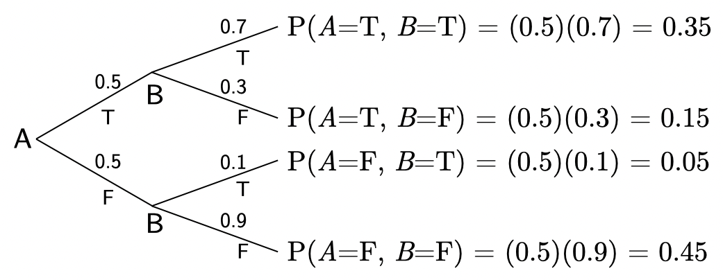
Below is a program that implements the following:
if A=true then { P(B{=}\mathtt{true}) = 0.7 }
if A=false then { P(B{=}\mathtt{true}) = 0.1 }
We can also write these relationships as conditional probabilities:
The table above shows the joint probability, {P(A, \, B)}.
Can you calculate these values based on the code for example_joint? Make sure that you can.
NoteSolution
Recovering latent probabilities from a joint distribution
Suppose we did not have access to the program that generated this table—we can see the joint distribution P(A, B), but we do not know the causal structure or the conditional probabilities that produced it. Can we recover the latent probabilities from the joint distribution alone?
Using only the table above, calculate the marginal probabilities {P(A{=}\mathtt{true})} and {P(B{=}\mathtt{true})}.
Using only the table above, calculate the conditional probabilities {P(B{=}\mathtt{true} \mid A{=}\mathtt{true})} and {P(B{=}\mathtt{true} \mid A{=}\mathtt{false})}.
This follows from the definition of conditional probability: {P(X \mid Y) = \frac{P(X, Y)}{P(Y)}} where {P(Y) > 0}.
Returning to treating example_joint as an explicit model that we defined, how could we modify example_joint to output the marginal and conditional probabilities?
@memodef example_marginal_a[_a: A](): agent: chooses(a in A, wpp=1) agent: chooses(b in B, wpp=( (0.7if b == {B.TRUE} else0.3 ) if a == {A.TRUE}else (0.1if b == {B.TRUE} else0.9 ) ))return Pr[agent.a == _a]_ = example_marginal_a(print_table=True)
Why doesn’t this give us the conditional distribution? Look at the table: it shows P(A{=}\mathtt{true}, \, B{=}b)—the joint probability restricted to the row where A{=}\mathtt{true}—not P(B \mid A{=}\mathtt{true}). These values don’t sum to 1 because we haven’t normalized by P(A{=}\mathtt{true}).
But the problem is deeper than normalization. In many PPLs, you could condition on a realized value of a random variable. But in memo, the agent itself chose the value of A—it has no uncertainty about its own choice, so there is nothing to condition on. Conditioning requires epistemic uncertainty: an agent who doesn’t know the value and must update their beliefs upon observing it. To express this in memo, we need to model a second agent whose choices the first agent is uncertain about.
Let’s say that the agent has a mental model of a friend’s choice of A and B:
@memodef mental_model_conditional_a[_a: A, _b: B](): agent: knows(_a, _b) agent: thinks[ friend: knows(_a, _b), friend: chooses(a in A, wpp=1), friend: chooses(b in B, wpp=( (0.7if b == {B.TRUE} else0.3 ) if a == {A.TRUE}else (0.1if b == {B.TRUE} else0.9 ) )), ]### condition the model agent: observes [friend.a] is _areturn agent[Pr[friend.a == _a, friend.b == _b]]_ = mental_model_conditional_a(print_table=True)
Now the agent doesn’t have inherent access to the friend’s knowledge about the state of A, but can observe it (e.g. if the friend shares that information).
By conditioning the model on an observed value of A, the model now computes a posterior distribution rather than a prior (unconditional) distribution. Whereas example_joint() computes the joint distribution {P(A, B)}, mental_model_conditional_a computes the conditional distribution {P(B \mid A)}—the posterior over B given the observed value of A.
Try removing one of the conditionals from the return statement. What do you get when the return statement is
agent[Pr[friend.a == _a, friend.b == _b]]
agent[Pr[friend.a == _a]]
agent[Pr[friend.b == _b]]
agent[Pr[friend.a]]
agent[Pr[friend.b]]
Now for each of these return statements, try removing _a: A and/or _b: B from the definition. Make sure you understand the effect of each modification (including why some combinations do not compile, and why others return redundant information or less information than you might want).
Statistical dependence
Suppose we observe that {A{=}\mathtt{true}}. What should we believe1 about B? From the program, {P(B{=}\mathtt{true} \mid A{=}\mathtt{true}) = 0.7}, which matches what we calculated above. If instead we observed {A{=}\mathtt{false}}, there’d be only a 10\% chance that {B{=}\mathtt{true}}.
The key observation: knowing something about A changes what we should believe about B. Different values of A yield different conditional distributions over B—that is, {P(B \mid A{=}\mathtt{true}) \neq P(B \mid A{=}\mathtt{false})}. This is the intuitive idea behind statistical dependence, which we define formally below.
The converse also holds: knowing the state of B updates what we should believe about A. Verify, using the joint distribution and the definition of conditional probability, that:
When information about one variable conveys information about another variable, the variables are statistically dependent.
We write this as {B \not\perp A}, where \perp denotes statistical independence and \not\perp denotes statistical dependence.
Defining statistical independence
What if knowing something about A never gave you information about B? Then the conditional distribution of B would be the same regardless of the value of A:
If this is the case, A and B are statistically independent: {B \perp A} (and thus {A \perp B})
In general, if {P(B \mid A) = P(B)}, then A and B are statistically independent, since information about A does not change the belief about B, i.e.:
P(B \mid A) = P(B) ~~\iff~~ B \perp A
The \iff symbol means “if and only if” (“iff”). I.e. {\spadesuit \iff \clubsuit} means that \spadesuit is only true and is always true if \clubsuit is true, and vice versa.
Recall the definition of conditional probability: {P(A \mid B) = \frac{P(A, B)}{P(B)}}, which can be rewritten as:
P(A, \, B) = P(B) \; P(A \mid B)
or the corollary
P(A, \, B) = P(A) \; P(B \mid A)
By substituting the relationship from above, { P(B \mid A) = P(B) ~~\iff~~ B \perp A }, into the definition of conditional probability, we arrive at the definition of statistical independence:
{P(A, \, B) = P(A) \; P(B) ~~\iff~~ A \perp B}
In other words,
A \perp B \\
\iff \\
P(A{=}a, \, B{=}b) = P(A{=}a) \; P(B{=}b) \\
~~\forall~~ (a, b) \in { \mathcal{A} \times \mathcal{B} }
The \forall symbol means “for all”, as in for every value that a and b can take.
If it is ever the case that this equality does not hold, then the random variables are statistically dependent (A \not\perp B):
A \not\perp B
~~~\text{if }~~ \\
{ P(A{=}a, \, B{=}b) \neq P(A{=}a) \; P(B{=}b) } \\
~~\text{ for some }~~ (a, b) \in \{ \mathcal{A} \times \mathcal{B} \}
Note that statistical dependence is symmetric: if A and B are statistically dependent, then {P(B \mid A) \neq P(B)}and{P(A \mid B) \neq P(A)}. Make sure you can show why this must be the case. (Hint: start from the definition of conditional probability and the factorization of the joint.)
Dependence vs correlation
“Statistical dependence” is not the same as “correlation.” When people say “correlation” they typically mean linear (Pearson) correlation, which measures only the strength of a linear relationship. Variables can be statistically dependent yet have zero linear correlation.
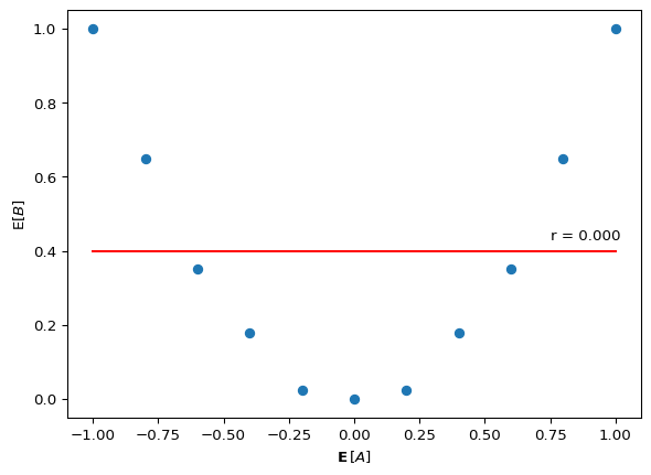
Consider the program below. B is causally dependent on A. Do you expect A and B to be statistically dependent? Do you expect A and B to be correlated? If you’re having trouble thinking through it, try drawing the shape of the data generated by the model. Once you’ve made your prediction, run the program.
from jax.scipy.stats.norm import pdf as normpdfA = jnp.linspace(-1, 1, 11)B = jnp.linspace(-1, 1.5, 11)@jax.jitdef B_pdf(b, a):return normpdf(b, a * a, 0.1)@memodef f[_a: A, _b: B](): agent: chooses(a in A, wpp=1) agent: chooses(b in B, wpp=B_pdf(b, a))return Pr[agent.a == _a, agent.b == _b]
NoteResult
res = f()def lobf(x, y):import numpy as npreturn (np.unique(x), np.poly1d(jnp.polyfit(x, y, 1))(np.unique(x)))def plot_results(x, y, ax=None, **kwargs):if ax isNone: fig, ax = plt.subplots() ax.scatter(x, y) _ = ax.set_xlabel(kwargs.get("xlabel", None)) _ = ax.set_ylabel(kwargs.get("ylabel", None))if"xlim"in kwargs: _ = ax.set_xlim(kwargs["xlim"])if"ylim"in kwargs: _ = ax.set_ylim(kwargs["ylim"]) ax.plot(*lobf(x, y), color="red") ax.text(0.75, 0.43, f"r = {jnp.corrcoef(x, y)[0,1]:0.3f}")b_ = jnp.array([jnp.dot(B, res[i, :]/res[i, :].sum()) for i inrange(len(A))])fig, ax = plt.subplots()plot_results(A, b_, ax=ax, xlabel=r"$\operatorname{\mathbf{E}} \left[ A \right]$", ylabel=r"$\operatorname{E}[B]$", xlim=(-1.1,1.1), ylim=(-0.05,1.05))
It should be clear that A and B are statistically dependent,2 but have a Pearson correlation of zero. (How would you prove that {A \not\perp B}? Hint: find specific values of a for which {P(B \mid A{=}a)} differs.)
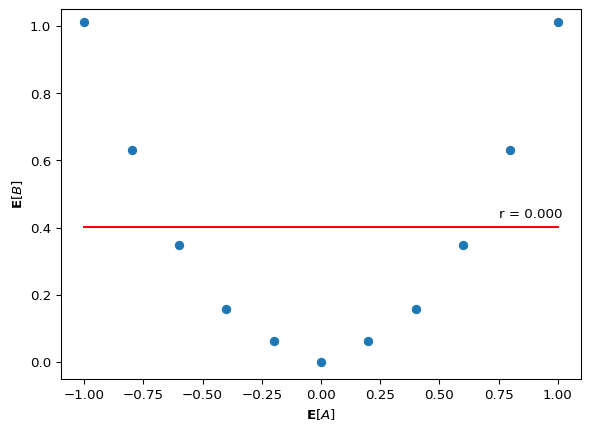
Compare the f program above to this one:
normpdfjit = jax.jit(normpdf)B0 = jnp.linspace(0, 1.2, 20)B = jnp.linspace(-0.5, 1.5, 20)C = jnp.array([-1, 1])A = jnp.linspace(-1, 1, 11)@memodef g[_a: A, _b: B](): agent: chooses(b0 in B0, wpp=1) agent: chooses(b in B, wpp=normpdfjit(b, b0, 0.1)) agent: chooses(c in C, wpp=1) agent: chooses(a in A, to_maximize=-abs(a - c * b0**0.5))return Pr[agent.a == _a, agent.b == _b]res = g()b_ = jnp.array([jnp.dot(B, res[i, :]/res[i, :].sum()) for i inrange(len(A))])fig, ax = plt.subplots()plot_results(A, b_, ax=ax, xlabel=r"$\mathbf{E}[A]$", ylabel=r"$\mathbf{E}[B]$", xlim=(-1.1,1.1), ylim=(-0.05,1.05))
In f, B causally depends on A (since B \sim \mathcal{N}(A^2, 0.1)). In g, A and B share a common cause (b0) but neither directly causes the other. These are different causal structures, yet they produce the same statistical signature: dependence between A and B with zero linear correlation.
To borrow a phrase from Richard McElreath (McElreath, 2020), the causes are not in the data. The joint distribution P(A, B) does not uniquely determine the causal structure that generated it.
Dependence can be context-specific
Statistical dependence is a global property: it is assessed over all possible values of the variables. But dependence can vanish in subsets of the data.
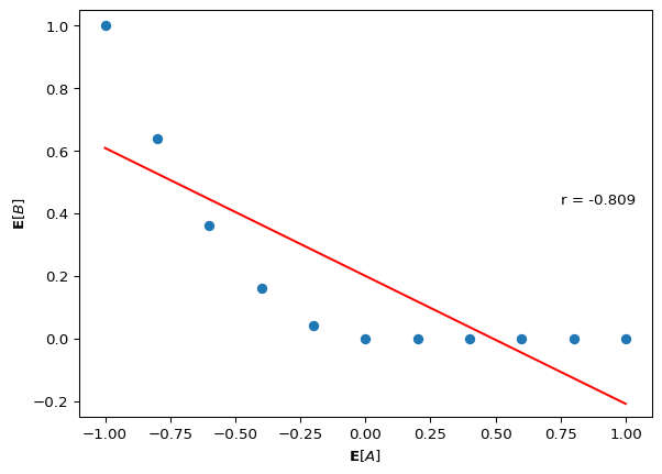
In the program below, A and B are statistically dependent (A \not\perp B) when assessed over their full support. However, if you restrict attention to the cases where A \geq 0, the relationship between A and B disappears—B no longer varies with A in that region.
normpdfjit = jax.jit(normpdf)A = jnp.linspace(-1, 1, 11)B = jnp.linspace(-0.5, 1.5, 20)@memodef h[_a: A, _b: B](): agent: chooses(a in A, wpp=1) agent: chooses(b in B, wpp=( normpdfjit(b, a**2, 0.1)if a <0else normpdfjit(b, 0, 0.1)))return Pr[agent.a == _a, agent.b == _b]res = h()fig, ax = plt.subplots()plot_results(A, jnp.array([jnp.dot(B, res[i, :]/res[i, :].sum()) for i inrange(len(A))]), ax=ax, xlabel=r"$\mathbf{E}[A]$", ylabel=r"$\mathbf{E}[B]$", xlim=(-1.1,1.1), ylim=(-0.25,1.05))
The important point: to determine whether {P(B \mid A) = P(B)}, we must check all possible values of A and B—not just those in a convenient subset. When we assert independence or dependence, we are making a claim over the entire support: P(B \mid A) = P(B) \;\; \forall \; (a,b) \in \mathcal{A} \times \mathcal{B}.
In causal inference, systematically examining a relationship across all levels of a variable is called stratification. Independence claims always implicitly require full stratification—a relationship that holds in a subset may not hold globally, and vice versa.
This points to one of the things that makes science hard. We don’t always know all of the causes, let alone measure them, let alone measure them at every possible value.
This is a central issue in trying to learn generative models by observing data. The causes are not in the data. In a more philosophical sense, is it even possible to observe a cause?3 If what our sense systems deliver are statistical regularities—patterns of co-occurrence, coincidence, correspondence, covariance, and association—how do people learn causally-structured mental models of the world and other minds? One view, developed by Gopnik, Tenenbaum, Griffiths and others (e.g. Gopnik et al., 2004; Griffiths & Tenenbaum, 2009; Tenenbaum et al., 2011), argues that evolution has equipped us with inductive biases—something like an abstract causal grammar—that constrain learning and enable children to acquire causal knowledge from sparse data. On this account, the prior over causal structures is itself innate (or at least matures early), even though the specific causal models are learned.
We have distinguished statistical dependence (a symmetric property of joint distributions) from causal dependence (a directed, structural property of generative processes). We have seen that different causal structures can produce identical joint distributions. In the next section, we examine how conditioning on additional variables can change the dependence relationships between other variables—creating dependence where there was none (explaining away), or removing it (screening off). These patterns are the key to understanding how evidence propagates through causal models.
Discussion
Consider the implications of these ideas for neural / connectionist models. If a feedforward network learns input-output mappings from data, what kind of “causal knowledge” can it represent? What are the limitations compared to a structured generative model?
Relate this to ideas we’ve discussed previously:
The role of overhypotheses and inductive constraints/biases in learning generative models. Consider Chomsky’s “poverty of the stimulus” argument: children acquire complex grammars from limited data, suggesting strong innate constraints on the hypothesis space.
The role of “enactive” or “embodied” cognition. How might the ability to causally intervene in the world—to push, pull, and manipulate objects—change the problem of learning from data? How does this relate to the “code interpreter” of ChatGPT, or to reinforcement learning from human feedback (RLHF)?
Is it possible to observe a cause? Suppose you observe me knock over my coffee cup. You see the cup fall, and you attribute it to my arm movement. But this attribution is itself an inference—one you learned to make by observing statistical regularities in how objects interact over your lifespan. At a more fundamental level, your perceptual system had to infer the spatial structure and physical properties of the scene, and that there are objects at all, from patterns of retinal stimulation—purely associative information.
Exercises
Joint distributions and marginals
Consider three equally-likely weather states (sunny, cloudy, rainy) and two equally-likely activities (indoors, outdoors). Write a memo model that computes the joint distribution P(\text{Weather}, \text{Activity}) assuming the two variables are independent. Verify from the output that P(W{=}w, A{=}a) = P(W{=}w) \; P(A{=}a) for all entries.
Now modify the model so that the activity depends on the weather: if sunny, P(\text{outdoors}) = 0.8; if cloudy, P(\text{outdoors}) = 0.5; if rainy, P(\text{outdoors}) = 0.1. From the joint distribution, compute (by hand) the marginal P(\text{Activity}). Are Weather and Activity statistically independent? Justify using the definition.
Conditioning in memo
Using the weather/activity model from the previous exercise, write a memo model with observes to compute the posterior P(\text{Weather} \mid \text{Activity}{=}\text{outdoors}). Which weather state is most likely given that the person is outdoors?
NoteHint
You need a two-agent model: an outer agent who has a mental model of a friend who chooses weather and activity. The agent then observes [friend.a] is _a, where _a is the query variable fixed to the outdoors value.
Revisit the example_joint model from the beginning of this chapter. Modify mental_model_conditional_a to condition on {A{=}\mathtt{false}} and return the full conditional distribution P(B \mid A{=}\mathtt{false}). Verify that P(B{=}\mathtt{true} \mid A{=}\mathtt{false}) = 0.1.
Hard constraints with observes_that
In addition to observes [X] is Y, which conditions on the equality of two random variables, memo provides observes_that[condition] for conditioning on arbitrary boolean expressions. This is a hard constraint: it sets the probability to zero for any outcome that violates the condition.
Write a memo model where a friend chooses an integer X uniformly from \{1, 2, \ldots, 10\}. The agent observes that the friend’s number is greater than 6. Return the posterior distribution P(X \mid X > 6). What should the result be? Verify your answer.
### uncomment and fill in# import jax.numpy as jnp# from memo import memo## X = jnp.arange(1, 11)## @memo# def ex_hard_constraint[_x: X]():# ...## _ = ex_hard_constraint(print_table=True)
The posterior should be uniform over \{7, 8, 9, 10\}, i.e. P(X{=}x \mid X > 6) = 0.25 for x \in \{7, 8, 9, 10\} and 0 otherwise.
Write a model where a friend draws two integers X, Y independently and uniformly from \{1, \ldots, 6\} (like rolling two dice). The agent observes that the sum X + Y = 7. Return the joint posterior P(X, Y \mid X + Y = 7).
There are 6 outcomes where X + Y = 7: (1,6), (2,5), (3,4), (4,3), (5,2), (6,1). Each has posterior probability 1/6.
Soft conditioning with observes_event
For noisy or continuous observations, memo provides observes_event(wpp=likelihood), which reweights outcomes by a non-negative likelihood function rather than zeroing them out:
This is analogous to factor(log_likelihood) or observe in WebPPL.
Suppose a friend picks a number \mu uniformly from \{0, 1, 2, \ldots, 10\}. You receive a noisy measurement of \mu: the observation is 5.5, with Gaussian noise of standard deviation 1.5. Write a memo model using observes_event to compute the posterior P(\mu \mid \text{observation}{=}5.5).
### uncomment and fill in# from jax.scipy.stats.norm import pdf as normpdf## Mu = jnp.arange(0, 11)## @memo# def noisy_obs[_mu: Mu]():# ...## _ = noisy_obs(print_table=True)
NoteSolution
from jax.scipy.stats.norm import pdf as normpdfMu = jnp.arange(0, 11)@memodef noisy_obs[_mu: Mu](): agent: knows(_mu) agent: thinks[ friend: knows(_mu), friend: chooses(mu in Mu, wpp=1), ] agent: observes_event(wpp=normpdf(5.5, friend.mu, 1.5))return agent[Pr[friend.mu == _mu]]_ = noisy_obs(print_table=True)
The posterior should peak at \mu = 5 and \mu = 6, with probabilities decreasing symmetrically away from 5.5.
Statistical dependence
Consider the following model. Without running it, determine whether C and D are statistically independent. Justify your answer by examining whether P(D \mid C) depends on the value of C. Then verify by running the model.
### uncomment to run# from enum import IntEnum# class C(IntEnum):# OFF = 0# ON = 1# class D(IntEnum):# OFF = 0# ON = 1## @memo# def cd_joint[_c: C, _d: D]():# agent: chooses(c in C, wpp=1)# agent: chooses(d in D, wpp=(# 0.6 if d == {D.ON} else 0.4# ))# return Pr[agent.c == _c, agent.d == _d]## _ = cd_joint(print_table=True)
NoteSolution
C and D are statistically independent. The wpp for D does not reference C at all, so P(D \mid C) = P(D) for all values of C. We can verify from the joint table: P(C{=}\texttt{ON}, D{=}\texttt{ON}) = 0.3 = 0.5 \times 0.6 = P(C{=}\texttt{ON}) \, P(D{=}\texttt{ON}), and similarly for all other cells.
Now modify the model above so that D depends on C: when C{=}\texttt{ON}, P(D{=}\texttt{ON}) = 0.9; when C{=}\texttt{OFF}, P(D{=}\texttt{ON}) = 0.2. Compute the joint, then condition on D{=}\texttt{ON} and compute the posterior P(C \mid D{=}\texttt{ON}). Compare this to the prior P(C). What does the comparison tell you?
From joint to conditional (by hand)
Consider a joint distribution over random variables X \in \{0, 1\} and Y \in \{0, 1, 2\} given by the following table:
Y{=}0
Y{=}1
Y{=}2
X{=}0
0.15
0.25
0.10
X{=}1
0.05
0.20
0.25
Compute P(X) and P(Y).
Compute P(Y \mid X{=}0) and P(Y \mid X{=}1).
Are X and Y statistically independent? Justify using the definition.
Compute P(X{=}1 \mid Y{=}2).
NoteRender env
%reset -fimport sysimport platformimport importlib.metadataprint("Python:", sys.version)print("Platform:", platform.system(), platform.release())print("Processor:", platform.processor())print("Machine:", platform.machine())print("\nPackages:")for name, version insorted( ((dist.metadata["Name"], dist.version) for dist in importlib.metadata.distributions()), key=lambda x: x[0].lower() # Sort case-insensitively):print(f"{name}=={version}")
Gopnik, Alison, Glymour, Clark, Sobel, David M., Schulz, Laura E., Kushnir, Tamar, & Danks, David. (2004). A theory of causal learning in children: Causal maps and Bayes nets. Psychological Review, 111(1), 3–32. https://doi.org/10.1037/0033-295X.111.1.3
Griffiths, Thomas L., & Tenenbaum, Joshua B. (2009). Theory-based causal induction. Psychological Review, 116(4), 661–716. https://doi.org/10.1037/a0017201
McElreath, Richard. (2020). Statistical rethinking: A Bayesian course with examples in R and Stan (Second edition). Chapman & Hall/CRC.
Tenenbaum, Joshua B., Kemp, Charles, Griffiths, Thomas L., & Goodman, Noah D. (2011). How to Grow a Mind: Statistics, Structure, and Abstraction. Science, 331(6022), 1279–1285. https://doi.org/10.1126/science.1192788
Footnotes
Here “belief” means credence—the probability mass a rational agent assigns to a proposition, given their information. This is the standard Bayesian usage, distinct from the binary notion of belief (believing something to be true or false) in epistemology.↩︎
The state of A changes what states of B are probable. E.g. if {A > 0.5} we expect the state of B to be greater than if {-0.1 < A < 0.1}. i.e. { \operatorname{\mathbf{E}} \left[ B \mid A > 0.5 \right] > \operatorname{\mathbf{E}} \left[ B \mid -0.1 < A < 0.1 \right] }↩︎
Philosophers including David Hume have argued against the observability of causation.↩︎