Causal models 1 - how do we know?
How do we know? / Statistical dependence
Statistical Dependence
Calculating joint probabilities
Recall what “causal (in)dependence” and “statistical (in)dependence” are (if you need a refresher, see the section on Dependence).
Let’s think more about what we mean by things being “statistically dependent”.
Below is a program that implements the following:
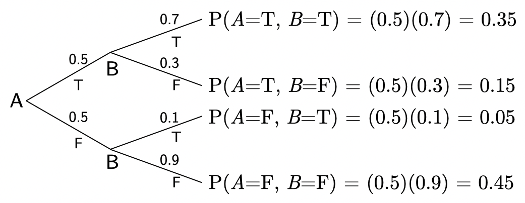
if A=true then \(P(B{=}\mathtt{true}) = 0.7\)
if A=false then \(P(B{=}\mathtt{true}) = 0.1\)
We can also write these relationships as conditional probabilities:
\[\begin{align} P(B{=}\mathtt{true} \mid A{=}\mathtt{true}) &= 0.7 \\ P(B{=}\mathtt{true} \mid A{=}\mathtt{false}) &= 0.1 \\ \end{align}\]Another way of writing the same is:
\[B \sim \text{Bernoulli}(p), p = \begin{cases} 0.7,& \text{if } A = true \\ 0.1, & \text{otherwise} \end{cases}\]For this example, we’ll say that \(P(A{=}\mathtt{true}) = 0.5\).
const truemodel = function() {
  const A = flip()
  const B = A ? flip(0.7) : flip(0.1)
  return { A, B }
}
const res = Infer({ method: 'enumerate' }, truemodel)
viz.table(res)
viz(res)
The above plot shows the joint probability, \(P(A, \, B)\).
Based on the code above, could you have predicted these values? Make sure that you can.
Solution
Calculating latent probabilities of a blackbox process
Let’s imagine running an experiment: we do not know the true generative process (i.e. the program), but we can observe the output of the process: tuples of \((a, \, b)\).
In other words, we do not know \(P(A)\), \(P(B \mid A)\), or the causal structure, but we can sample from the blackbox model.
By making repeated observations, we can calculate the probability of observing different tuples (i.e. combinations of \(a\) and \(b\)). Here’s a program that simulates us making \(100000\) observations from the model and calculating the probability of each tuple:
const blackbox = function() {
  const A = flip()
  const B = A ? flip(0.7) : flip(0.1)
  return { A, B }
}
const res = Infer({ method: 'forward', samples: 100000 }, blackbox)
viz.table(res)
If we sample many observations from the blackbox generative process, we’ll end up with approximately these values:
| \(a\) | \(b\) | \(P(A{=}a, \, B{=}b)\) |
|---|---|---|
| \(\mathtt{true}\) | \(\mathtt{true}\) | \(0.35\) |
| \(\mathtt{true}\) | \(\mathtt{false}\) | \(0.15\) |
| \(\mathtt{false}\) | \(\mathtt{true}\) | \(0.05\) |
| \(\mathtt{false}\) | \(\mathtt{false}\) | \(0.45\) |
Can we recover the latent probabilities that generated these data? Using only the table above, calculate \(P(B{=}\mathtt{true} \mid A{=}\mathtt{true})\) and \(P(B{=}\mathtt{true} \mid A{=}\mathtt{false})\)?
Solution
$$ P(B{=}\mathtt{true} \mid A{=}\mathtt{true}) = \frac{P(B{=}\mathtt{true}, \, A{=}\mathtt{true})}{P(A{=}\mathtt{true})} = \frac{0.35}{0.5} = 0.7 $$ This follows from the definition of conditional probability: $$p(x, y) = p(y) \, p(x \mid y)$$What about the marginal distributions? Using the joint probabilities from the table, calculate \(P(A{=}\mathtt{true})\) and \(P(B{=}\mathtt{true})\).
Solution
$$ P(A{=}\mathtt{true}) = \sum_{b \in B} P(A{=}\mathtt{true}, B{=}b) = P(A{=}\mathtt{true}, \, B{=}\mathtt{true}) + P(A{=}\mathtt{true}, \, B{=}\mathtt{false}) = 0.35 + 0.15 = 0.5 $$ $$ P(B{=}\mathtt{true}) = \sum_{a \in A} P(B{=}\mathtt{true}, \, A{=}a) = P(B{=}\mathtt{true}, \, A{=}\mathtt{true}) + P(B{=}\mathtt{true}, \, A{=}\mathtt{false}) = 0.35 + 0.05 = 0.4 $$ This follows from the law of total probability: $$P(X) = \sum_{y} P(X, \, Y{=}y)$$ or equivalently: $$P(X) = \sum_{y} P(Y{=}y) \, P(X \mid Y{=}y)$$Ok, so by making repeated observations of a blackbox generative process, we can estimate the joint probability of the observed variables. And from the joint probability of the data, we can calculate statistical properties of the unknown generative process.
Calculating latent probabilities by conditioning a model
Let’s now say that we have a model of the generative process. Here is the same generative structure as the truemodel above. How could we modify truemodel to output the conditional and marginal probabilities?
One way to get the conditional probabilities is to condition the model.
Here is a modified program that outputs \(P(B \mid A{=}\mathtt{true})\) by conditioning the generative process on A:
const model = function() {
  const A = flip()
  const B = A ? flip(0.7) : flip(0.1)
  condition(A) // this is the same as condition(A === true)
  return { A, B }
}
const res = Infer({ method: 'enumerate' }, model)
viz.table(res)
viz(res)
Modify this program to condition on A being false to see that \(P(B{=}\mathtt{true} \mid A{=}\mathtt{false}) = 0.1\).
Defining statistical dependence
Say we sample a single tuple from this model and observe that \(A{=}\mathtt{true}\). What do we think the value of \(B\) is in that tuple? Since \(P(B{=}\mathtt{true} \mid A{=}\mathtt{true}) = 0.7\), we should think that there’s a \(70\%\) chance that the tuple is \((A{=}\mathtt{true}, \, B{=}\mathtt{true})\). However, if we drew a tuple where \(A{=}\mathtt{false}\), there’d be a \(10\%\) chance that \(B{=}\mathtt{true}\).
Notice that: knowing something about \(A\) changes the belief about \(B\).
This is the same as saying that \(B\) depends statistically on \(A\).
Or equivalently, that different realizations of \(A\) change \(P(B \mid A)\).
We write this using a symbol that means “not orthogonal”: \(B \not\perp A\).
We can also show that \(A\) depends statistically on \(B\), by conditioning on \(B\).
(Remember, \(A\) is statistically dependent on \(B\) if information about \(B\) changes the belief about \(A\). So we can check for statistical dependence by testing if \(B\) taking any value changes the probability of \(A\) taking any value.)
const model_AgivenB = function() {
  const A = flip()
  const B = A ? flip(0.7) : flip(0.1)
  condition(B)
  return A
}
const model_AgivennotB = function() {
  const A = flip()
  const B = A ? flip(0.7) : flip(0.1)
  condition(!B) // this is the same as condition(B === false)
  return A
}
const res_AgivenB = Infer({ method: 'enumerate' }, model_AgivenB)
const res_AgivennotB = Infer({ method: 'enumerate' }, model_AgivennotB)
viz(res_AgivenB, {
  xLabel: 'A',
  yLabel: 'P(A|B=true)',
})
viz(res_AgivennotB, {
  xLabel: 'A',
  yLabel: 'P(A|B=false)',
})
In other words, knowing something about \(B\) changes the belief about \(A\), and knowing something about \(A\) changes the belief about \(B\).
It is true in general that statistical dependence is symmetric. Writing \(B \not\perp A\) is the same as writing \(A \not\perp B\). So rather than saying “\(A\) depends statistically on \(B\)”, we just say “\(A\) and \(B\) are statistically dependent”.
Defining statistical independence
What if knowing something about \(A\) gave you no information about \(B\)?
In that case, \(P(B \mid A{=}\mathtt{true}) = P(B \mid A{=}\mathtt{false})\). And if \(A\) was a different RV, this would hold true for any value that \(A\) could take.
Since the value of \(A\) does not change the probability of \(B\), \(P(B \mid A) = P(B)\).
In general, if \(P(B \mid A) = P(B)\) then \(A\) and \(B\) are statistically independent (\(A \perp B\) and \(B \perp A\)).
Recall the definition of conditional probability: \(P(A \mid B) = \frac{P(A, B)}{P(B)}\), which can be rewritten as:
\[P(A, B) = P(B) \, P(A \mid B)\]and also as
\[P(A, B) = P(A) \, P(B \mid A)\]Based on what we have just concluded, we can then go on to say \(P(B \mid A) = P(B)\) iff \(A \perp B\). By substituting this into the above definition, we arrive at the definition of statistical independence.
\[P(A, B) = P(A) P(B) \text{ iff } A \perp B\]Similarly, \(P(B \mid A) \neq P(B)\) iff \(A \not\perp B\).
Dependence vs correlation
Is “statistical dependence” the same as “correlation”? No. Things that are statistically dependent can be correlated or uncorrelated.
Consider the program below. B is causally dependent on A. Do you expect A and B to be statistically dependent? Do you expect A and B to be correlated? If you’re having trouble thinking through it, try drawing what shape data generated by the model will form. Once you’ve made your predictions, run the program.
const model1 = function() {
  const A = uniform(-1, 1)
  const B = A * A + gaussian(0, 0.1)
  return { A, B }
}
const res = Infer({ method: 'forward', samples: 1000 }, model1)
viz(res)
It should be clear that A and B are statically dependent$^{right?}$, but have a correlation of approximately zero. (How would you prove that \(A \not\perp B\)?)
right? The value of \(A\) changes what values of \(B\) are likely. E.g. if \(A < 0.5\) you’d expect the value of \(B\) to be greater than if \(-0.1 < A < 0.1\).
Compare the model1 program above to this one:
const model2 = function() {
  const B0 = uniform(0, 1)
  const B = B0 + gaussian(0, 0.1)
  const C = flip() ? -1 : 1
  const A = C * Math.pow(B0, 0.5)
  return { A, B }
}
const res = Infer({ method: 'forward', samples: 1000 }, model2)
viz(res)
In model1, B is causally dependent on A, whereas in model2, B is causally independent of A. But you can’t tell that from the data.
In other words, the causes are not in the data (a phrase from Richard McElreath).
Contextual dependence
const model = function() {
  const A = uniform(-1, 1)
  const B = A < 0 ? A * A + gaussian(0, 0.1) : gaussian(0, 0.1)
  return { A, B }
}
const res = Infer({ method: 'forward', samples: 1000 }, model)
viz(res)
In this program, \(A\) and \(B\) are statistically dependent (\(A \not\perp B\)). But, if you only examined the relationship between \(A\) and \(B\) when \(A\) is positive, it would look like \(A\) and \(B\) are statistically independent (\(A \perp B\)).
An important point here is that, in order to determine if \(P(B \mid A) = P(B)\), we need to assess all possible values of \(A\).
This is called stratification, and it’s implied when we talk about (in)dependence.
Here’s another example. In this case, \(B\) depends on \(A\) in general. But, \(B\) is independent of \(A\) when \(C \leq 0.5\). So, to determine if \(P(B \mid A) = P(B)\), we need to assess not only all possible values of \(A\), but also all other variables that have a causal effect on \(A\) or \(B\).
const model = function() {
  const C = gaussian(0, 1)
  const A = uniform(-1, 1)
  const B = C > 0.5 ? A * A + gaussian(0, 0.1) : gaussian(0, 0.1)
  return { A, B }
}
const res = Infer({ method: 'forward', samples: 1000 }, model)
viz(res)
This points to one of the things that makes science hard. We don’t always know all of the causes, let alone measure them, let alone measure them at every possible value.
This is a central issue in trying to learn generative models by observing data. The causes are not in the data. In a more philosophical sense, is even possible to observe a cause?
This also points to how the practice of building causal models can help us think though data collection and analysis. Writing out an ontological model of the processes that you’re studying helps you think about: What are the relevant variables? Are you measuring the right variables in the ways you need to in order to ask the questions that you want to?
Discussion
- What this means for neural / connectionist models.
- Relate this to ideas we’ve discussed previously:
- The role of overhypotheses and inductive constraints/biases in learning generative models. Consider Chomsky’s notion of “poverty of the stimulus”.
- The role “enactive”/”embodied” cognition. How might the ability to causally intervene in the world change the problem of learning from data? How does this relate to things like the “code interpreter” of chatGPT? To reinforcement learning from human feedback (RLHF) in deep learning?
- In philosophical sense, is possible to observe a cause? Say that you observe me knock over my coffee cup. Sure, you saw me have a causal effect on my coffee cup. But you had to learn to make that causal inference by observing the statistical regularities of how objects interact over your lifespan. You inferred the causal relationship between my movement and the movement of the coffee cup, and you had to learn to make that causal inference. At a more fundamental level, you’re needing to infer the spatial structure and physical properties of the objects, and that there are objects, based on patterns of retinal transductions—purely associative information.
Causal Dependence
What we’ve seen so far is that we may be able to deduce statistical (in)dependence between some variables.
However, if we cannot repeatedly measure all of the variables at all of the values that may effect some variables of interest, there is no guarantee that we’d be able to deduce the statistical (in)dependence from data alone. This is, of course, the case for most real-world processes.
Moreover, even if we can deduce statistical (in)dependence for a set of variables, that does not tell us what the causal relationships are.
So how might we try to learn causal relationships?
Well, we can causally intervene in a process and measure the effects.
Detecting Dependence Through Intervention
In the preceding examples, I have intentionally used variables that do not imply specific causal relationships (e.g. using \(A\) and \(B\) rather than \(disease\) and \(symptom\)). This was to underscore how statistical dependence is symmetric and does not specify causal relationships. We now turn to causal dependence.
Onward :: Causal Dependence.
Next lecture notes: 10. Day 10 - Intuitive causal reasoning