import numpy as np
from matplotlib import pyplot as plt
def wavelength_to_rgb(wavelength_nm, gamma=0.8):
"""Convert wavelength (nm) to RGB using Dan Bruton's algorithm.
This is the canonical algorithm used by Wikipedia and most spectrum
visualizations. Source: http://www.physics.sfasu.edu/astro/color/spectra.html
"""
wl = wavelength_nm
# Piecewise linear RGB assignment
if 380 <= wl < 440:
r = (440 - wl) / (440 - 380)
g = 0.0
b = 1.0
elif 440 <= wl < 490:
r = 0.0
g = (wl - 440) / (490 - 440)
b = 1.0
elif 490 <= wl < 510:
r = 0.0
g = 1.0
b = (510 - wl) / (510 - 490)
elif 510 <= wl < 580:
r = (wl - 510) / (580 - 510)
g = 1.0
b = 0.0
elif 580 <= wl < 645:
r = 1.0
g = (645 - wl) / (645 - 580)
b = 0.0
elif 645 <= wl <= 780:
r = 1.0
g = 0.0
b = 0.0
else:
r = g = b = 0.0
# Intensity falloff at edges of visible spectrum
if 380 <= wl < 420:
factor = 0.3 + 0.7 * (wl - 380) / (420 - 380)
elif 420 <= wl <= 700:
factor = 1.0
elif 700 < wl <= 780:
factor = 0.3 + 0.7 * (780 - wl) / (780 - 700)
else:
factor = 0.0
# Apply intensity factor and gamma correction
r = (r * factor) ** gamma
g = (g * factor) ** gamma
b = (b * factor) ** gamma
return np.array([r, g, b])
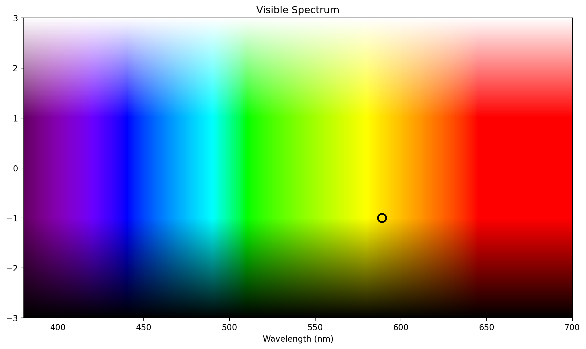
def plot_visible_spectrum(wavelength_range=(380, 700), resolution=300):
"""Plot the visible spectrum with gradient overlays for lightness.
X-axis: wavelength in nm
Y-axis: ranges from -3 to 3
Pure spectral colors throughout, with white gradient overlay (y=1 to 3)
and black gradient overlay (y=-1 to -3).
"""
wavelengths = np.linspace(wavelength_range[0], wavelength_range[1], resolution)
# Build the base spectrum image (same color for all rows)
image = np.zeros((resolution, resolution, 3))
for j, wl in enumerate(wavelengths):
rgb = wavelength_to_rgb(wl)
image[:, j] = rgb
fig_, ax_ = plt.subplots(figsize=(10, 6))
extent = [wavelength_range[0], wavelength_range[1], -3, 3]
# Plot the base spectrum
ax_.imshow(image, aspect='auto', extent=extent)
# White gradient overlay (y=1 to y=3, alpha 0 to 1)
white_gradient = np.ones((resolution, resolution, 4)) # RGBA white
for i in range(resolution):
y = 3 - 6 * i / (resolution - 1) # row to y mapping
if y > 1:
alpha = (y - 1) / 2 # 0 at y=1, 1 at y=3
else:
alpha = 0
white_gradient[i, :, 3] = alpha
ax_.imshow(white_gradient, aspect='auto', extent=extent)
# Black gradient overlay (y=-1 to y=-3, alpha 0 to 1)
black_gradient = np.zeros((resolution, resolution, 4)) # RGBA black
for i in range(resolution):
y = 3 - 6 * i / (resolution - 1) # row to y mapping
alpha = (-1 - y) / 2 if y < -1 else 0
black_gradient[i, :, 3] = alpha
ax_.imshow(black_gradient, aspect='auto', extent=extent)
ax_.set_xlabel('Wavelength (nm)')
# ax_.set_ylabel('y')
ax_.set_title('Visible Spectrum')
# ax_.axhline(y=1, color='white', linestyle='--', alpha=0.3, linewidth=0.5)
# ax_.axhline(y=-1, color='white', linestyle='--', alpha=0.3, linewidth=0.5)
plt.tight_layout()
return fig_, ax_
fig, ax = plot_visible_spectrum()
ax.scatter(589, -1, s=100, edgecolor="k", facecolor="none", linewidth=2)