Bayesian Inference: Parametric and Non-Parametric Posterior Distributions

Jupyter Notebook

• Jupyter Notebook

NB the Jupyter notebook includes interactive widgets that are very useful for building an understanding of these models.

Problem

Consider a simple likelihood model: data are normally distributed with mean \mu and standard deviation \sigma.

We draw three observations (d \in \mathcal{D}) from this data-generating process:

\mathcal{D} = \{ -5, 5, 10\}

Given these data, we wish to infer \mu, assuming a fixed standard deviation \sigma (e.g. \sigma = 5).

From Bayes’ rule, we know:

\begin{align*} P(\mu \mid \mathcal{D}) = \frac{P(\mu) ~ P(\mathcal{D} \mid \mu)}{P(\mathcal{D})} = \frac{P(\mu) ~ P(\mathcal{D} \mid \mu)}{\int_{\mu} P(\mu) ~ P(\mathcal{D} \mid \mu) ~\mathrm{d}\mu} \end{align*}

Where:

• P(\mu) is the prior belief about \mu before observing any data
• P(\mathcal{D} \mid \mu) is the likelihood of observing the data under a given hypothesis
• P(\mathcal{D}) is the marginal likelihood of the data

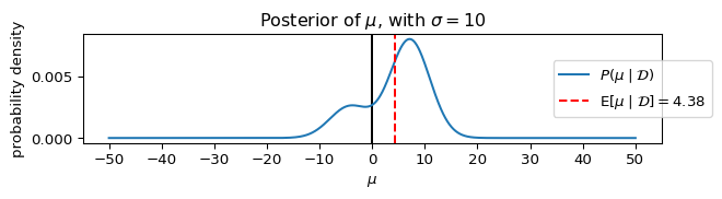
Model with bimodal prior

Imagine that we have a prior belief that the data generating process could have a mean near 10, or a mean near -10. We can instantiate this bimodal belief as a Gaussian mixture with equal weights on two components:

Thus, the model is defined as:

\begin{align*} \mu &\sim 0.5 \cdot \mathcal{N}(-10, 5) + 0.5 \cdot \mathcal{N}(10, 5) \\ \sigma &= 5 \quad \text{(fixed)} \\ d &\sim \mathcal{N}(\mu, \sigma) \end{align*}

Prior

P(\mu) = 0.5 \cdot \mathcal{N}(\mu \mid -10, 5) + 0.5 \cdot \mathcal{N}(\mu \mid 10, 5)

Likelihood

P(\mathcal{D} \mid \mu) = \prod_{d \in \mathcal{D}} \mathcal{N}(d \mid \mu, \sigma)

Posterior

P(\mu \mid \mathcal{D}) = \frac{P(\mu) \cdot P(\mathcal{D} \mid \mu)}{\int P(\mu) \cdot P(\mathcal{D} \mid \mu) \,\mathrm{d}\mu}

Implementation

We can implement this model in memo like so:

import jax
import jax.numpy as jnp
from memo import memo
from jax.scipy.stats.norm import pdf as normpdf
from jax.scipy.stats.norm import logpdf as normlogpdf

Data = jnp.array([-5, 5, 10])

Mu = jnp.linspace(-50, 50, 1000)

@jax.jit
def prior(mu):
    component1 = normpdf(mu, loc=-10, scale=5)
    component2 = normpdf(mu, loc=10, scale=5)
    return jnp.mean(jnp.array([component1, component2]))

@jax.jit
def likelihood(mu, sigma=5):
    return jnp.exp(jnp.sum(normlogpdf(Data, loc=mu, scale=sigma)))

@memo
def model_bimodal_prior[
    _mu: Mu,
](sigma=1):
    observer: knows(_mu)
    observer: thinks[
        ### consider a hypothesis ###
        process: given(mu in Mu, wpp=prior(mu)), ### given the hypothesis, mu
    ]

    ### score the observed data under the likelihood model ###
    observer: observes_event(wpp=likelihood(process.mu, sigma))

    ### return the posterior probability of mu ###
    return observer[Pr[process.mu == _mu]]

Interactive Visualization

Let’s plot the posterior, P(\mu \mid \mathcal{D}), assuming different values for \sigma.

from matplotlib import pyplot as plt


def plot_model(sigma=1, figsize=(5, 4), verbose=False):
    posterior = model_bimodal_prior(sigma=sigma)
    fig, ax = plt.subplots(figsize=figsize)
    ax.axvline(0, color="black", linestyle="-")
    ax.plot(Mu, posterior, label=r"$P(\mu \mid \mathcal{D})$")
    mu_expectation = jnp.dot(Mu, posterior)
    ax.axvline(
        mu_expectation, 
        color='red', 
        linestyle='--', 
        label=r"$\operatorname{E}" + r"[\mu \mid \mathcal{D}]=" + f"{mu_expectation:6.2f}$")
    _ = ax.set_xticks(jnp.arange(-50, 50 + 10, 10))
    _ = ax.set_title(rf"Posterior of $\mu$, with $\sigma={sigma}$")
    _ = ax.legend(bbox_to_anchor=(0.8, 0.5), loc='center left')
    _ = ax.set_xlabel(r"$\mu$")
    _ = ax.set_ylabel("probability density")

    plt.tight_layout()
    plt.show()

param_list = [
    dict(sigma=1),
    dict(sigma=5),
    dict(sigma=10),
    dict(sigma=20),
]
for i_params_, params_ in enumerate(param_list):
    plot_model(**params_, figsize=(7, 2))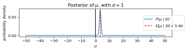

Exercise

Replace the bimodal prior with a Gaussian prior. First implement a Gaussian prior with mean 0 and standard deviation 5. Then try different standard deviations. Describe how the Gaussian prior affects the inferred posterior.

Solution

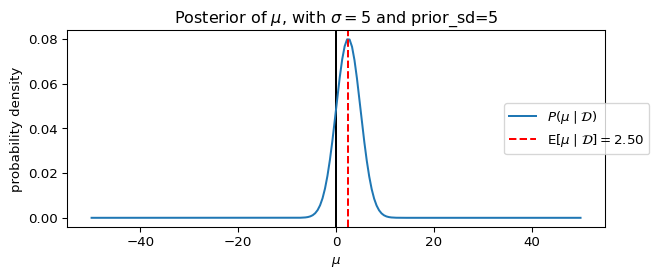
Model with Gaussian prior

The model is defined as:

\begin{align*} \mu &\sim \mathcal{N}(0, 5) \\ \sigma &= 5 \quad \text{(fixed)} \\ d &\sim \mathcal{N}(\mu, \sigma) \end{align*}

Prior

P(\mu) = \mathcal{N}(\mu \mid 0, 5)

Likelihood

P(\mathcal{D} \mid \mu) = \prod_{d \in \mathcal{D}} \mathcal{N}(d \mid \mu, \sigma)

Posterior

P(\mu \mid \mathcal{D}) = \frac{P(\mu) \cdot P(\mathcal{D} \mid \mu)}{P(\mathcal{D})} = \frac{\mathcal{N}(\mu \mid 0, 5) \cdot \prod_{d \in \mathcal{D}} \mathcal{N}(d \mid \mu, \sigma)}{\int \mathcal{N}(\mu \mid 0, 5) \cdot \prod_{d \in \mathcal{D}} \mathcal{N}(d \mid \mu, \sigma) \,\mathrm{d}\mu}

In contrast to the bimodal prior model, with a Gaussian prior and Gaussian likelihood (when inferring the mean with an assumed variance), the posterior is also Gaussian. This is a classic example of conjugate priors where the posterior belongs to the same parametric family as the prior.

The posterior distribution in this case can be derived analytically as:

P(\mu \mid \mathcal{D}) = \mathcal{N}(\mu \mid \mu_n, \sigma_n)

where:

\begin{align*} \mu_n &= \frac{\sigma^2 \mu_0 + n \sigma_0^2 \bar{d}}{\sigma^2 + n \sigma_0^2} \\ \sigma_n^2 &= \frac{\sigma_0^2 \sigma^2}{\sigma^2 + n \sigma_0^2} \end{align*}

Here:

• \mu_0 and \sigma_0^2 are the prior mean and variance (0 and 5^2 in this case)
• \bar{d} is the sample mean of the data (approximately 3.33 in this case)
• n is the number of observations (3 in this case)
• \sigma^2 is the assumed variance of the likelihood (5^2 in this case)

This illustrates an important distinction: while many posterior distributions don’t have a simple parametric form (as in the bimodal prior example), some specific combinations of priors and likelihoods do result in parametric posteriors.

Implementation

import jax
import jax.numpy as jnp
from memo import memo
from jax.scipy.stats.norm import pdf as normpdf

Data = jnp.array([-5, 5, 10])

Mu = jnp.linspace(-50, 50, 200)

@jax.jit
def prior(mu, scale=5):
    return normpdf(mu, loc=0, scale=scale)

@jax.jit
def likelihood(mu, sigma=5):
    return jnp.prod(normpdf(Data, loc=mu, scale=sigma))

@memo
def model_gaussian_prior[
    _mu: Mu,
](sigma=1, prior_sd=5):
    observer: knows(_mu)
    observer: thinks[
        ### consider a hypothesis ###
        ### (hypotheses are normally distributed a priori) ###
        process: given(mu in Mu, wpp=prior(mu, prior_sd)), ### given the hypothesis, mu
    ]

    ### score the observed data under the likelihood model ###
    observer: observes_event(
        wpp=likelihood(process.mu, sigma)
    )

    ### return the posterior probability of mu ###
    return observer[Pr[process.mu == _mu]]

Visualizing the Gaussian Prior Results

We can visualize the posterior distribution for the Gaussian prior model using the same plotting function defined earlier:

from matplotlib import pyplot as plt


def plot_model_gaussian_prior(sigma=1, prior_sd=5, figsize=(5, 4), verbose=False):
    posterior = model_gaussian_prior(sigma=sigma, prior_sd=prior_sd)
    fig, ax = plt.subplots(figsize=figsize)
    ax.axvline(0, color="black", linestyle="-")
    ax.plot(Mu, posterior, label=r"$P(\mu \mid \mathcal{D})$")
    mu_expectation = jnp.dot(Mu, posterior)
    ax.axvline(
        mu_expectation, 
        color='red', 
        linestyle='--', 
        label=r"$\operatorname{E}" + r"[\mu \mid \mathcal{D}]=" + f"{mu_expectation:6.2f}$")
    _ = ax.set_title(rf"Posterior of $\mu$, with $\sigma={sigma}$ and prior_sd={prior_sd}")
    _ = ax.legend(bbox_to_anchor=(0.8, 0.5), loc='center left')
    _ = ax.set_xlabel(r"$\mu$")
    _ = ax.set_ylabel("probability density")

    plt.tight_layout()
    plt.show()

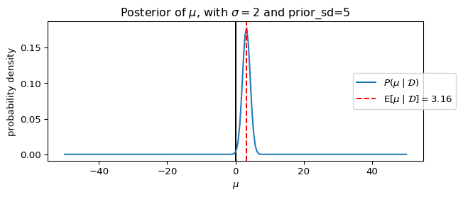
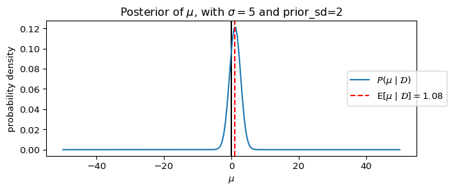
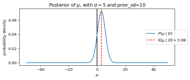
param_list = [
    dict(sigma=20, prior_sd=5),
    dict(sigma=5, prior_sd=5),
    dict(sigma=2, prior_sd=5),
    dict(sigma=5, prior_sd=2),
    dict(sigma=5, prior_sd=10),
]
for params_ in param_list:
    plot_model_gaussian_prior(**params_, figsize=(7, 3))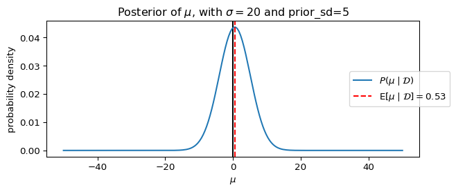

---

Render env

%reset -f
import sys
import platform
import importlib.metadata

print("Python:", sys.version)
print("Platform:", platform.system(), platform.release())
print("Processor:", platform.processor())
print("Machine:", platform.machine())

print("\nPackages:")
for name, version in sorted(
    ((dist.metadata["Name"], dist.version) for dist in importlib.metadata.distributions()),
    key=lambda x: x[0].lower()  # Sort case-insensitively
):
    print(f"{name}=={version}")

Python: 3.13.3 | packaged by conda-forge | (main, Apr 14 2025, 20:44:30) [Clang 18.1.8 ]
Platform: Darwin 23.6.0
Processor: arm
Machine: arm64

Packages:
annotated-types==0.7.0
anyio==4.9.0
appnope==0.1.4
argon2-cffi==23.1.0
argon2-cffi-bindings==21.2.0
arrow==1.3.0
astroid==3.3.10
asttokens==3.0.0
async-lru==2.0.5
attrs==25.3.0
babel==2.17.0
beautifulsoup4==4.13.4
bleach==6.2.0
certifi==2025.4.26
cffi==1.17.1
cfgv==3.4.0
charset-normalizer==3.4.2
click==8.2.0
comm==0.2.2
contourpy==1.3.2
cycler==0.12.1
debugpy==1.8.14
decorator==5.2.1
defusedxml==0.7.1
dill==0.4.0
distlib==0.3.9
executing==2.2.0
fastjsonschema==2.21.1
filelock==3.18.0
fonttools==4.58.0
fqdn==1.5.1
h11==0.16.0
httpcore==1.0.9
httpx==0.28.1
identify==2.6.10
idna==3.10
importlib_metadata==8.7.0
ipykernel==6.29.5
ipython==9.2.0
ipython_pygments_lexers==1.1.1
ipywidgets==8.1.7
isoduration==20.11.0
isort==6.0.1
jax==0.6.0
jaxlib==0.6.0
jedi==0.19.2
Jinja2==3.1.6
joblib==1.5.0
json5==0.12.0
jsonpointer==3.0.0
jsonschema==4.23.0
jsonschema-specifications==2025.4.1
jupyter-cache==1.0.1
jupyter-events==0.12.0
jupyter-lsp==2.2.5
jupyter_client==8.6.3
jupyter_core==5.7.2
jupyter_server==2.16.0
jupyter_server_terminals==0.5.3
jupyterlab==4.4.2
jupyterlab_pygments==0.3.0
jupyterlab_server==2.27.3
jupyterlab_widgets==3.0.15
kiwisolver==1.4.8
MarkupSafe==3.0.2
matplotlib==3.10.3
matplotlib-inline==0.1.7
mccabe==0.7.0
memo-lang==1.2.0
mistune==3.1.3
ml_dtypes==0.5.1
nbclient==0.10.2
nbconvert==7.16.6
nbformat==5.10.4
nest-asyncio==1.6.0
networkx==3.4.2
nodeenv==1.9.1
notebook_shim==0.2.4
numpy==2.2.6
opt_einsum==3.4.0
optype==0.9.3
overrides==7.7.0
packaging==25.0
pandas==2.2.3
pandas-stubs==2.2.3.250308
pandocfilters==1.5.1
parso==0.8.4
pexpect==4.9.0
pillow==11.2.1
platformdirs==4.3.8
plotly==5.24.1
pre_commit==4.2.0
prometheus_client==0.22.0
prompt_toolkit==3.0.51
psutil==7.0.0
ptyprocess==0.7.0
pure_eval==0.2.3
pycparser==2.22
pydantic==2.11.4
pydantic_core==2.33.2
Pygments==2.19.1
pygraphviz==1.14
pylint==3.3.7
pyparsing==3.2.3
python-dateutil==2.9.0.post0
python-dotenv==1.1.0
python-json-logger==3.3.0
pytz==2025.2
PyYAML==6.0.2
pyzmq==26.4.0
referencing==0.36.2
requests==2.32.3
rfc3339-validator==0.1.4
rfc3986-validator==0.1.1
rpds-py==0.25.0
ruff==0.11.10
scikit-learn==1.6.1
scipy==1.15.3
scipy-stubs==1.15.3.0
seaborn==0.13.2
Send2Trash==1.8.3
setuptools==80.7.1
six==1.17.0
sniffio==1.3.1
soupsieve==2.7
SQLAlchemy==2.0.41
stack-data==0.6.3
tabulate==0.9.0
tenacity==9.1.2
terminado==0.18.1
threadpoolctl==3.6.0
tinycss2==1.4.0
toml==0.10.2
tomlkit==0.13.2
tornado==6.5
tqdm==4.67.1
traitlets==5.14.3
types-python-dateutil==2.9.0.20250516
types-pytz==2025.2.0.20250516
typing-inspection==0.4.0
typing_extensions==4.13.2
tzdata==2025.2
uri-template==1.3.0
urllib3==2.4.0
virtualenv==20.31.2
wcwidth==0.2.13
webcolors==24.11.1
webencodings==0.5.1
websocket-client==1.8.0
widgetsnbextension==4.0.14
xarray==2025.4.0
zipp==3.21.0