Multilevel models

Jupyter Notebook

• Jupyter Notebook

NB the Jupyter notebook includes interactive widgets that are very useful for building an understanding of these models.

Human minds naturally organize concepts and categories hierarchically. While every individual dog is unique, we also learn about how different breeds look and behave, just as we learn about how

Hierarchical models allow us to capture the shared latent structure underlying observations of multiple related concepts, processes, or systems – to abstract out the elements in common to the different sub-concepts, and to filter away uninteresting or irrelevant differences.

The Departmental Tardiness Problem

Imagine that your university hires a new president. On her first week, she schedules a meeting with professors from three departments, Government (G), English (E), and Mathematics (M). The Government professor arrives 1 minute late, the English professor arrives 15 minutes early, and the Mathematics professor arrives 30 minutes late. From this single meeting the new president updates her beliefs about when professors will show up to scheduled meetings. But how should the president update her beliefs?

This scenario exemplifies a fundamental challenge in inductive inference: How should one balance learning about specific entities (individual departments) versus more abstract patterns (professors as a population)? Should the president expect Mathematics professors to arrive late, or is this observation merely a chance occurrence? Should she expect all professors to have unpredictable arrival times, or might there be statistical regularities within and between departments?

Multilevel models

A model that infers information about the population without differentiating subpopulations is doing “complete variance pooling”, meaning that all of the variance in the data is treated as being generated by the same distribution. I.e. the data is pooled together and treated as iid observations drawn from a single distribution.

If the president thinks of each department independently, what she learns about the tardiness of professors from one department will not change her expectation about professors from other departments. In this case, there would be “no variance pooling” between departments. The president’s observations of the three professors have no bearing on her belief about what to expect of a professor from a fourth department (e.g. Psychology).

“Partial variance pooling” models represent uncertainty at multiple levels of abstraction. Based on her observation from this meeting, the president will update her beliefs about these departments and the greater population. In other words, what she observes about the Math department might strongly update her beliefs about that department, moderately update her beliefs about the broader population, and that in turn could weakly update her beliefs about the English department.

Complete pooling

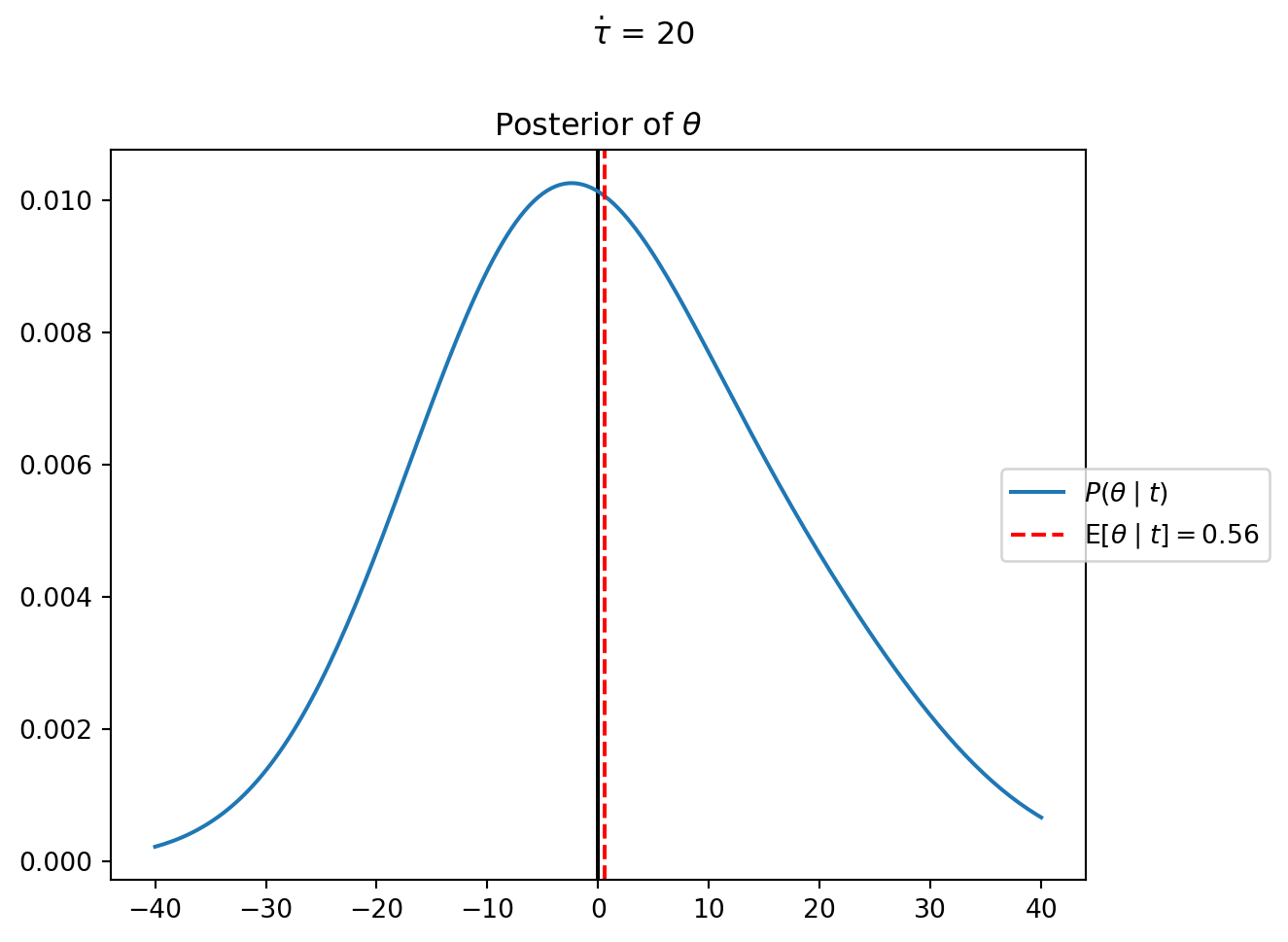
Let’s build a complete pooling model of the president’s belief about the punctuality of professors without distinguishing between departments. In this model, we posit a single parameter θ representing the “typical” arrival time for professors (positive values indicating lateness, negative values indicating earliness), with variation around this central tendency. The president observes data { t = \langle t_G, t_E, t_M \rangle = \langle 1, -15, 30 \rangle }.

We’ll model the president’s belief about the greater population of professors as a normal distribution centered at \theta with standard deviation \dot\sigma. Prior to meeting with anyone, the president thinks that professors will, on average, show up on time, but that some will show up early and some late. We can encode this prior belief as a normal distribution centered at zero, with some standard deviation, let’s say 20. I.e. the prior for \theta is:

\theta ~\sim~ \mathcal{N}\left( \dot{\mu}{=}0, \dot{\tau}{=}20 \right)

…v Here, θ follows a prior normal distribution centered at 0 (reflecting an initial belief that professors typically arrive on time) with standard deviation 20 (reflecting substantial uncertainty). Each observed arrival time follows a normal distribution centered on θ with standard deviation 15 minutes (reflecting the expected variability in individual behavior).

Let’s implement this model using probabilistic programming: …^

If she observes that professors tend to be late, then her posterior estimate of \theta will have an expected value greater than zero (i.e. { \operatorname{E}[\theta \mid t] > 0 }), and if she ends up expecting professors to be early, then { \operatorname{E}[\theta \mid t] < 0 }.

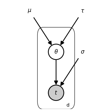
In this tutorial I’ll use the dot above to indicate that a variable is fixed, not inferred (the dot is not standard notation, just what I’m using here). In the graphical schematic, fixed parameters are depicted as bare symbols rather than nodes. Note that “fixed” means the values are not updated during inference (but you can, of course, manually tune these values or learn suitable values by minimizing some loss function in conjunction with a model fitting algorithm).

Since the model infers the distribution of \theta, the graphical schematic depicts it as an open node (i.e. a latent random variable). The data in this model are t.

We specify the likelihood as,

t_d ~\sim~ \mathcal{N}(\theta, \dot\sigma{=}15)

I.e., for whatever the true value of \theta is for the population of professors, the president thinks that when professors actually show up will follow a normal distribution, centered on the true value of \theta, with standard deviation 15.

Complete Variance Pooling

\begin{align*} \theta ~\sim&~ \mathcal{N}\left( \dot{\mu}{=}0, \dot{\tau}{=}20 \right) \\ t_d ~\sim&~ \mathcal{N}(\theta, \dot\sigma{=}15) \\ d ~\in&~ D,~~~ \text{where}~~~ D = \{ \text{G}, \text{E}, \text{M} \} \end{align*}

%reset -f
import jax
import jax.numpy as jnp
from memo import memo
from enum import IntEnum
from jax.scipy.stats.norm import pdf as normpdf
from jax.scipy.stats.cauchy import pdf as cauchypdf
from matplotlib import pyplot as plt

normpdfjit = jax.jit(normpdf)

class Department(IntEnum):
    GOVERNMENT = 0
    ENGLISH = 1
    MATH = 2

t = jnp.array([1, -15, 30])
sigma = 15

Theta = jnp.linspace(-40, 40, 200)

@jax.jit
def professor_arrival_likelihood(d, theta):
    ### likelihood of a professor from department d 
    ### showing up t_d minutes early/late, 
    ### for a given theta and sigma.
    return normpdf(t[d], theta, sigma)

@memo
def complete_pooling[
    _theta: Theta,
](mu=0, tau=1):
    president: knows(_theta)
    president: thinks[
        department: chooses(d in Department, wpp=1),
        department: chooses(theta in Theta, wpp=normpdfjit(theta, mu, tau))
    ]
    president: observes_event(
        wpp=professor_arrival_likelihood(department.d, department.theta))
    return president[Pr[department.theta == _theta]]

mu_ = 0
tau_ = 20
res = complete_pooling(mu=mu_, tau=tau_)

### check the size and sum of the output
# res.shape
# res.sum()

fig, ax = plt.subplots()

ax.axvline(0, color="black", linestyle="-")
theta_posterior = res
theta_expectation = jnp.dot(Theta, theta_posterior)
ax.plot(Theta, theta_posterior, label=r"$P(\theta \mid t)$")
ax.axvline(
    theta_expectation, 
    color='red', 
    linestyle='--', 
    label=(
        r"$\operatorname{E}"
        + rf"[\theta \mid t]={theta_expectation:0.2f}$")
)
_ = ax.set_title(r"Posterior of $\theta$")
_ = ax.legend(bbox_to_anchor=(0.9, 0.5), loc='center left')

_ = plt.suptitle(fr"$\dot\tau$ = {tau_}", y=1)
plt.tight_layout()
plt.show()

Try changing the data to t = jnp.array([-20, -10, 30]). Notice how changing the data for one group updates the expectation of the population.

This model captures how a cognitive agent might form a single prototype for “professor punctuality,” aggregating information across all observations without distinguishing between departments. It parallels how humans might form a basic-level category representation by abstracting across instances—for example, forming a general concept of “dog” that captures central tendencies across different breeds while ignoring breed-specific variations.

The key limitation of this single-level representation is its inability to capture systematic between-group differences. If Mathematics professors genuinely tend to arrive late while English professors tend to arrive early, this model fails to represent this structure, treating departmental differences as random noise rather than meaningful patterns.

No Pooling: Independent Representations

… At the opposite extreme, we might maintain entirely separate representations for each department, with no connections between them. This approach, termed no pooling, treats each department as a distinct inference problem. …

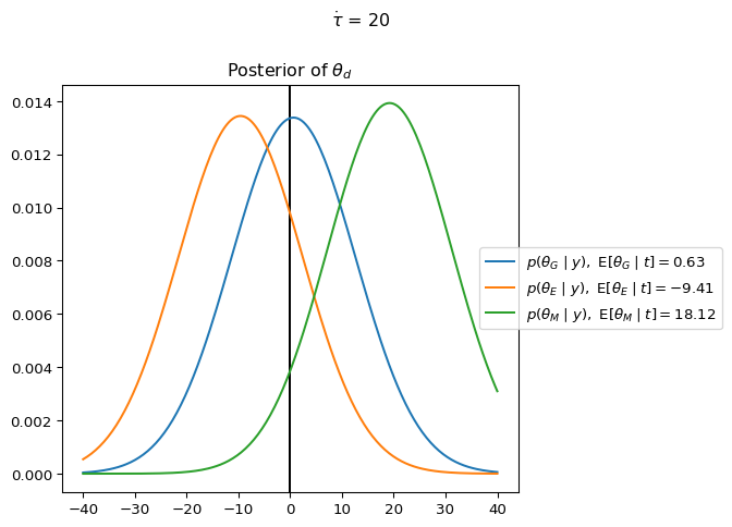
In contrast to complete pooling, which assumes all observations are generated by a shared population-level distribution parameterized by \theta, the no pooling model treats each department as having its own independent parameter \theta_d. The key change is that instead of having a single \theta drawn from the prior distribution, we now have three independent parameters \theta_G, \theta_E, and \theta_M.

The practical meaning of this change is significant:

In complete pooling, an observation of the Math professor being late would shift our expectations for all departments. In no pooling, learning that the Math professor is late only updates our beliefs about the Math department. Each department’s parameter is estimated using only data from that department.

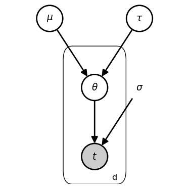
The key change in our model specification is that we have replaced the single \theta with three parameters, \theta_d.

No Variance Pooling

\begin{align*} \theta_d ~\sim&~ \mathcal{N}\left( \dot{\mu}{=}0, \dot{\tau}{=}20 \right) \\ t_d ~\sim&~ \mathcal{N}(\theta_d, \dot\sigma{=}15) \\ d ~\in&~ D,~~~ \text{where}~~~ D = \{\text{G}, \text{E}, \text{M} \} \end{align*}

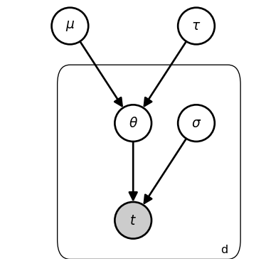
The plate (rectangular box) with label d indicates that everything inside is repeated for each department d \in D. Variables inside the plate have a unique value for each department. Variables outside the plate are shared across all departments.

To change the complete_pooling model to the no_pooling model we make a simple change, adding the conditional statement

president: observes [department.d] is _d

and the query variable _d in the definition, [_d: Department, ...].

%reset -f
import jax
import jax.numpy as jnp
from memo import memo
from enum import IntEnum
from jax.scipy.stats.norm import pdf as normpdf
from jax.scipy.stats.cauchy import pdf as cauchypdf
from matplotlib import pyplot as plt

normpdfjit = jax.jit(normpdf)

class Department(IntEnum):
    GOVERNMENT = 0
    ENGLISH = 1
    MATH = 2

t = jnp.array([1, -15, 30])
sigma = 15

Theta = jnp.linspace(-40, 40, 200)

@jax.jit
def professor_arrival_likelihood(d, theta):
    ### likelihood of a professor from department d 
    ### showing up t_d minutes early/late, 
    ### for a given theta and sigma.
    return normpdf(t[d], theta, sigma)

@memo
def no_pooling[
    _d: Department,
    _theta: Theta,
](mu=0, tau=1):
    president: knows(_theta)
    president: thinks[
        department: chooses(d in Department, wpp=1),
        department: chooses(theta in Theta, wpp=normpdfjit(theta, mu, tau))
    ]
    president: observes [department.d] is _d ### new conditional statement
    president: observes_event(
        wpp=professor_arrival_likelihood(department.d, department.theta))
    return president[Pr[department.theta == _theta]]

mu_ = 0
tau_ = 20
res = no_pooling(mu=mu_, tau=tau_)

### check the size and sum of the output
# res.shape
# res.sum()
# res[0].sum()
# res[1].sum()
# res[2].sum()

fig, ax = plt.subplots()

ax.axvline(0, color="black", linestyle="-")
for d in Department:
    department_name = d.name
    department_abbrev = department_name[0]
    theta_posterior = res[d]
    theta_expectation = jnp.dot(Theta, theta_posterior)
    ax.plot(
        Theta, 
        theta_posterior, 
        label=(
            rf"$p(\theta_{department_abbrev} \mid y),~ "
            + r"\operatorname{E}"
            + rf"[\theta_{department_abbrev} \mid t]={theta_expectation:0.2f}$")
    )
_ = ax.set_title(r"Posterior of $\theta_d$")
_ = ax.legend(bbox_to_anchor=(0.9, 0.5), loc='center left')

_ = plt.suptitle(fr"$\dot\tau$ = {tau_}", y=1)
plt.tight_layout()
plt.show()

Try changing the data to t = jnp.array([-20, -15, 30]). Notice how changing the data for one group does not affect the expectation of the posterior of the other groups.

Previously, the complete_pooling model returned an array of shape (200,) with 200 being the size of the sample space of Theta. With the addition of the conditional statement, what array shape does no_pooling return? Make sure you understand the shape change, what each dimension reflects, and why the values sum in the ways that they do.

The key theoretical distinction is that in no pooling, we’re asserting that the timing behavior of professors in different departments is independent of the behavior of professors from other departments (i.e. when professors from one department show up for meetings carries no information about when professors from a different department will show up). This is an unrealistically strong assumption.

The no_pooling and complete_pooling models highlight an important practical tradeoff: no pooling can better capture differences between departments but may suffer from high variance in its estimates due to small sample sizes within each department. Complete pooling has lower variance but may miss important systematic differences between departments.

…vvv The key addition is president: observes [department.d] is _d, which conditions on a specific department. This model maintains separate representations for each department, with no information transfer between them.

This approach corresponds to maintaining separate subordinate-level concepts without forming more abstract generalizations. It would be analogous to learning about Dalmatians, Golden Retrievers, and Beagles as entirely distinct categories without ever forming an integrated concept of “dog” that captures their shared characteristics.

With limited data per department, these separate representations will exhibit high variance. The model fails to leverage potential patterns that might exist across departments, making inefficient use of the available evidence. …^^^

Partial pooling

In partial pooling, every observation updates beliefs across multiple levels of abstraction. The critical insight is that while departments may differ in their typical timing behavior, the departments are not statistically independent. They are influenced by common causes. To model the president’s reasoning about these multiple levels of uncertainty, we modify the no_pooling model by adding priors over \mu and \tau.

…v The most sophisticated approach recognizes that while departments may have distinctive characteristics, they likely share certain commonalities (being composed of academics within the same institution). This approach, termed partial pooling, maintains representations at multiple levels of abstraction simultaneously, connecting them through a hierarchical structure.

Here, μ represents the institution-wide typical arrival time, while τ represents the between-department variability. Each department’s θ_d is drawn from this institution-wide distribution rather than from an independent prior. …^

Rather than being fixed values, \mu and \tau become latent parameters to be jointly inferred alongside \theta_d.

The higher-level latent parameters \mu and \tau characterize a “population-level” distribution from which department-specific \theta_d values are generated.

The key change to the model is that rather than { \theta_d ~\sim~ \mathcal{N}\left( \dot{\mu}{=}0, \dot{\tau}{=}20 \right) }, we have { \theta_d ~\sim~ \mathcal{N}\left(\mu, \tau \right) } and specify hyperpriors on these new latent parameters: { \mu ~\sim~ \mathcal{N}(0, \dot\sigma_{\mu}) } and { \tau ~\sim~ \text{HalfCauchy}(\dot\sigma_{\tau}) }.

Note that there are new fixed parameters: mu_scale ({ \dot\sigma_\mu}) and tau_scale ({ \dot\sigma_\tau }), but I am omitting there from the graphical schematic for the sake of visual simplicity.

Partial Variance Pooling

\begin{align*} \mu ~\sim&~ \mathcal{N}(0, \dot\sigma_{\mu}) \\ \tau ~\sim&~ \text{HalfCauchy}(\dot\sigma_{\tau}) \\ \theta_d ~\sim&~ \mathcal{N}\left(\mu, \tau \right) \\ t_d ~\sim&~ \mathcal{N}(\theta_d, \dot\sigma{=}15) \\ d ~\in&~ D,~~~ \text{where}~~~ D = \{\text{G}, \text{E}, \text{M} \} \end{align*}

%reset -f
import jax
import jax.numpy as jnp
from memo import memo
from enum import IntEnum
from jax.scipy.stats.norm import pdf as normpdf
from jax.scipy.stats.cauchy import pdf as cauchypdf
from matplotlib import pyplot as plt

normpdfjit = jax.jit(normpdf)

class Department(IntEnum):
    GOVERNMENT = 0
    ENGLISH = 1
    MATH = 2

t = jnp.array([1, -15, 30])
sigma = 15

Mu = jnp.linspace(-25, 25, 100)  ### sample space for new hyperprior
Tau = jnp.linspace(1, 30, 100)  ### sample space for new hyperprior
Theta = jnp.linspace(-40, 40, 200)

### PDF for new hyperprior
@jax.jit
def half_cauchy(x, scale=1.0):
    return 2 * cauchypdf(x, 0, scale)

@jax.jit
def professor_arrival_likelihood(d, theta):
    ### likelihood of a professor from department d 
    ### showing up t_d minutes early/late, 
    ### for a given theta and sigma.
    return normpdf(t[d], theta, sigma)

@memo
def department_model[_mu: Mu, _tau: Tau](d):
    department: knows(_mu, _tau)
    department: chooses(theta in Theta, wpp=normpdfjit(theta, _mu, _tau))
    return E[ department[professor_arrival_likelihood(d, theta)] ]

@memo
def partial_pooling[_mu: Mu, _tau: Tau](mu_scale=5, tau_scale=5):
    president: knows(_mu, _tau)
    president: thinks[
        population: chooses(mu in Mu, wpp=normpdfjit(mu, 0, mu_scale)),
        population: chooses(tau in Tau, wpp=half_cauchy(tau, tau_scale)),
    ]

    president: observes_event(
        wpp=department_model[population.mu, population.tau]({Department.GOVERNMENT}))
    president: observes_event(
        wpp=department_model[population.mu, population.tau]({Department.ENGLISH}))
    president: observes_event(
        wpp=department_model[population.mu, population.tau]({Department.MATH}))

    return president[Pr[population.mu == _mu, population.tau == _tau]]

Let’s think about what each variable represents.

The likelihood model professor_arrival_likelihood gives the probability that a professor from department d shows up t_d minutes early/late, under a given \theta_d and \sigma:

t_d ~\sim~ \mathcal{N}(\theta_d, \dot\sigma{=}15)

We can write the likelihood as { P(t_d \mid \theta_d, \mu, \tau ; \sigma) }. The marginal posterior { P(\theta_d \mid t) } will thus represent the president’s belief about the true value of \theta_d for a given department d.

…vvv This model maintains representations at two levels of abstraction: 1. The institution-wide distribution characterized by μ and τ 2. The department-specific tendencies captured by θ_d

This hierarchical approach mirrors the structure of human conceptual knowledge, which typically spans multiple levels of abstraction. We understand both that “mammals generally have fur” (a superordinate-level generalization) and that “dogs typically bark” (a basic-level generalization).

When estimated from our data, this model produces department-specific inferences that are “regularized” toward the population mean—an effect termed “shrinkage.” The extent of this regularization depends on the inferred between-department variability (τ) and the amount of evidence available for each department.

Shrinkage and Statistical Information Transfer

A key phenomenon in hierarchical models is shrinkage—the tendency for group-specific estimates to be pulled or “shrunk” toward the overall population mean. The magnitude of shrinkage depends on several factors:

1. Sample size: Departments with more observations experience less shrinkage
2. Between-department variance (τ): When τ is small (departments are similar), shrinkage is stronger
3. Within-department variance (σ): When σ is large (noisy observations), shrinkage is stronger

To extract the department-specific estimates: …^^^

@memo
def department_model_theta[_theta: Theta](d, mu_scale, tau_scale):
    obs: thinks[
        department: chooses(mu in Mu, tau in Tau, wpp=partial_pooling[mu, tau](mu_scale, tau_scale)),
        department: chooses(theta in Theta, wpp=normpdfjit(theta, mu, tau))
    ]
    obs: observes_event(wpp=professor_arrival_likelihood(d, department.theta))
    obs: knows(_theta)
    return obs[Pr[department.theta == _theta]]

def plot_model(mu_scale=1, tau_scale=1, figsize=(10, 8), verbose=False):
    posterior = partial_pooling(mu_scale=mu_scale, tau_scale=tau_scale)

    # Marginal over Tau (sum over Mu)
    posterior_tau = posterior.sum(axis=0)
    # Marginal over Mu (sum over Tau)
    posterior_mu = posterior.sum(axis=1)

    fig, axs = plt.subplots(3, 1, figsize=figsize)

    ax = axs[0]
    ax.axvline(0, color="black", linestyle="-")
    ax.plot(Mu, posterior_mu, label=r"$P(\mu \mid t)$")
    mu_expectation = jnp.dot(Mu, posterior_mu)
    ax.axvline(
        mu_expectation, 
        color='red', 
        linestyle='--', 
        label=r"$\operatorname{E}" + rf"[\mu \mid t]={mu_expectation:0.2f}$")
    _ = ax.set_title(r"Posterior of $\mu$")
    _ = ax.legend(bbox_to_anchor=(0.9, 0.5), loc='center left')

    ax = axs[1]
    ax.axvline(0, color="black", linestyle="-")
    ax.plot(Tau, posterior_tau, label=r"$P(\tau \mid t)$")
    tau_expectation = jnp.dot(Tau, posterior_tau)
    ax.axvline(
        tau_expectation, 
        color='red', 
        linestyle='--', 
        label=r"$\operatorname{E}" + rf"[\tau \mid t]={tau_expectation:0.2f}$")
    _ = ax.set_title(r"Posterior of $\tau$")
    _ = ax.legend(bbox_to_anchor=(0.9, 0.5), loc='center left')

    ax = axs[2]
    ax.axvline(0, color="black", linestyle="-")
    for d in Department:
        department_name = d.name
        department_abbrev = department_name[0]
        theta_posterior = department_model_theta(d, mu_scale, tau_scale)
        theta_expectation = jnp.dot(Theta, theta_posterior)
        ax.plot(
            Theta, 
            theta_posterior, 
            label=(
                rf"$P(\theta_{department_abbrev} \mid t),~ " 
                + r"\operatorname{E}" 
                + rf"[\theta_{department_abbrev} \mid t]={theta_expectation:0.2f}$"))
    _ = ax.set_title(r"Posterior of $\theta_d$")
    _ = ax.legend(bbox_to_anchor=(0.9, 0.5), loc='center left')

    _ = plt.suptitle(f"mu_scale = {mu_scale}, tau_scale = {tau_scale}", y=1)
    plt.tight_layout()
    plt.show()

    if verbose:
        for d in Department:
            department_name = d.name
            department_abbrev = department_name[0]
            theta_posterior = department_model_theta(d, mu_scale, tau_scale)
            posterior_mean = jnp.average(Theta, weights=theta_posterior)
            posterior_second_moment = jnp.average(Theta**2, weights=theta_posterior)
            posterior_variance = posterior_second_moment - posterior_mean**2
            print(f"{mu_scale=}, {tau_scale=} : E[θ{department_abbrev} | t]={posterior_mean:0.3f}, Var[θ{department_abbrev} | t]={posterior_variance:0.3f}")

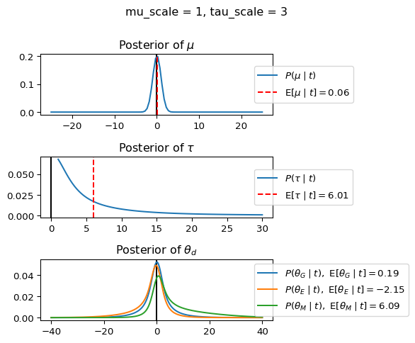
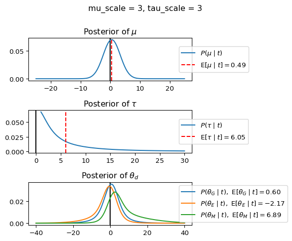
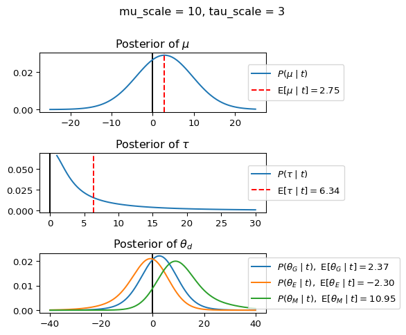
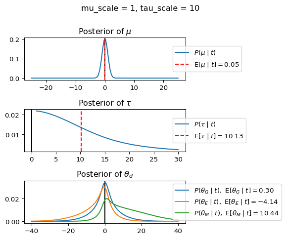
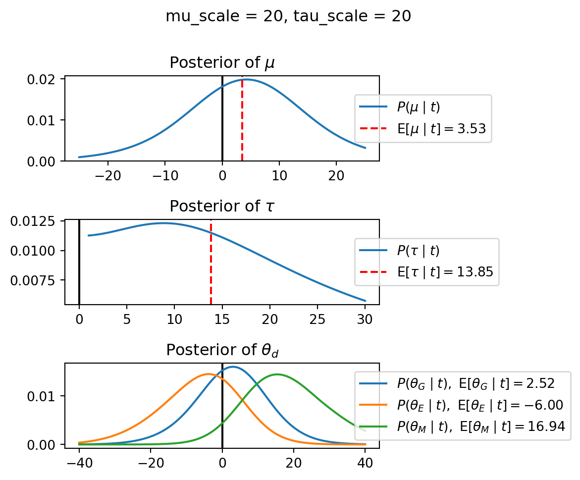
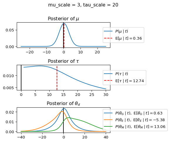
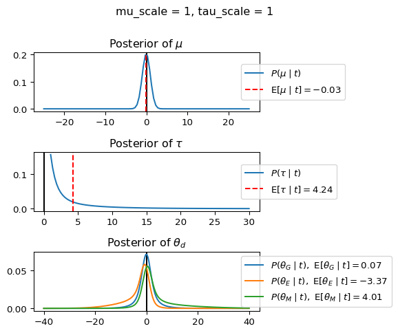
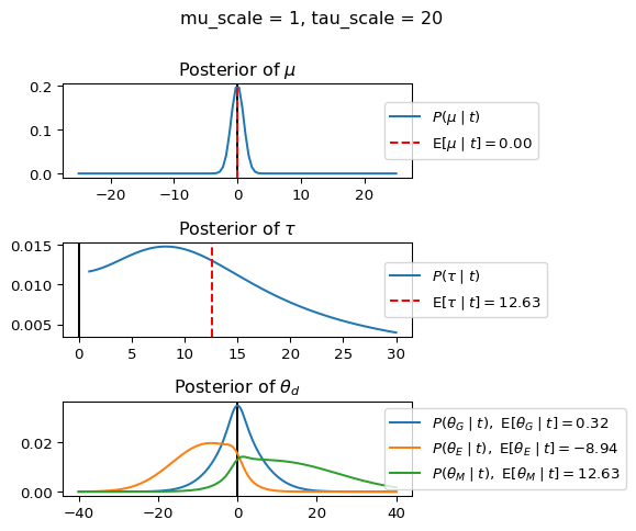
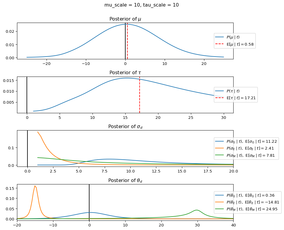
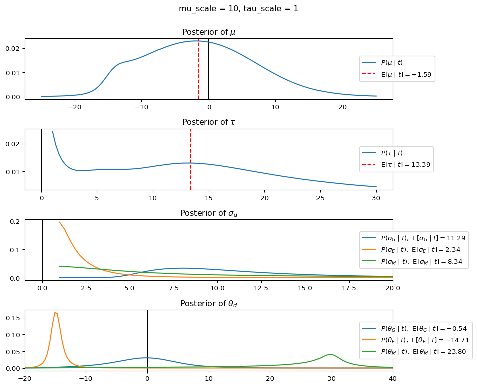
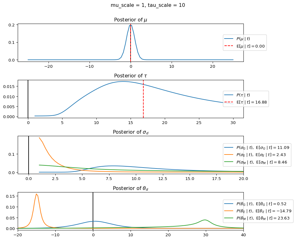
When mu_scale is small (e.g. { \dot\sigma_{\mu}{=}1 }) the location of the distribution over \theta_d will be centered near zero. When mu_scale is large (e.g. { \dot\sigma_{\mu}{=}10 }), the center of { \mathcal{N}(\mu, \tau) } can move to new locations with greater freedom. This results in a more flexible population-level mean, allowing the model to adapt to data that suggests professors generally arrive early or late across all departments. With a large mu_scale, the model places less prior constraint on where the overall population mean should be, letting the data have more influence on determining this parameter.

param_list = [
    dict(mu_scale=1, tau_scale=3),
    dict(mu_scale=3, tau_scale=3),
    dict(mu_scale=10, tau_scale=3),
]
for i_params_, params_ in enumerate(param_list):
    plot_model(**params_, figsize=(6, 5), verbose=True)

mu_scale=1, tau_scale=3 : E[θG | t]=0.187, Var[θG | t]=29.778
mu_scale=1, tau_scale=3 : E[θE | t]=-2.155, Var[θE | t]=40.307
mu_scale=1, tau_scale=3 : E[θM | t]=6.092, Var[θM | t]=82.286

mu_scale=3, tau_scale=3 : E[θG | t]=0.595, Var[θG | t]=35.435
mu_scale=3, tau_scale=3 : E[θE | t]=-2.168, Var[θE | t]=46.285
mu_scale=3, tau_scale=3 : E[θM | t]=6.891, Var[θM | t]=79.738

mu_scale=10, tau_scale=3 : E[θG | t]=2.370, Var[θG | t]=61.138
mu_scale=10, tau_scale=3 : E[θE | t]=-2.297, Var[θE | t]=73.436
mu_scale=10, tau_scale=3 : E[θM | t]=10.948, Var[θM | t]=80.582

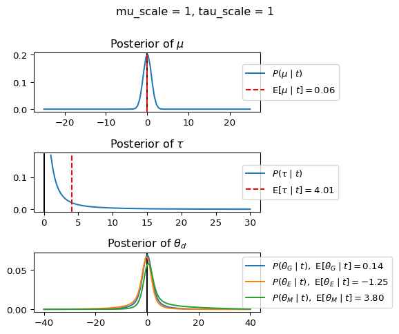
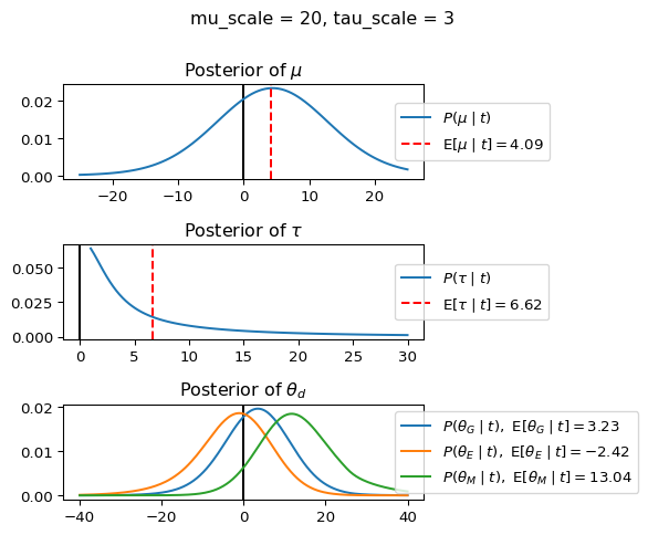
When tau_scale is small (e.g. { \dot\sigma_{\tau}{=}1 }), the distribution { \theta_d ~\sim~ \mathcal{N}(\mu, \tau) } will be narrow, which will result in strong shrinkage of department-specific means toward the overall population mean. This effectively reduces the differences between departments, making the model behave more like the complete pooling model. The practical interpretation is that the model assumes departments are relatively homogeneous in their timing behavior.

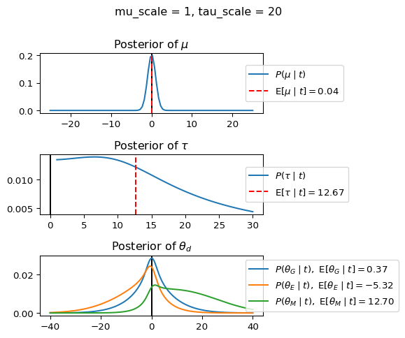
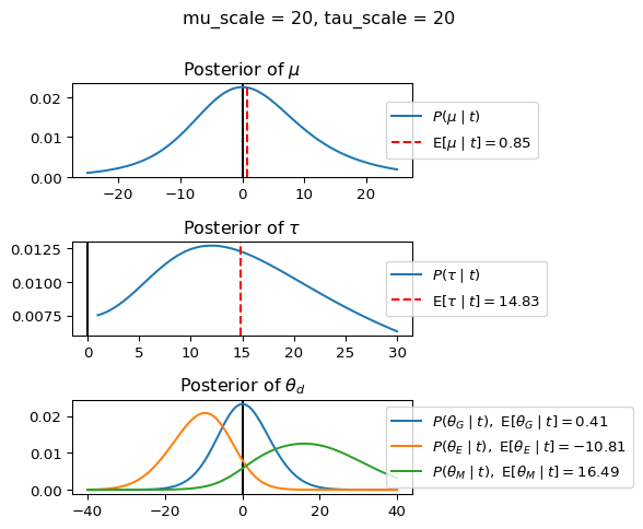
When tau_scale is large (e.g. { \dot\sigma_{\tau}{=}20 }), the { \theta_d } can diverge more freely from the population mean, resulting in weaker shrinkage effects. Department-specific estimates will be closer to their empirical means and less influenced by data from other departments. This allows the model to capture more heterogeneity between departments, making it behave more like the no pooling model while still maintaining some information sharing.

param_list = [
    dict(mu_scale=1, tau_scale=1),
    dict(mu_scale=1, tau_scale=3),
    dict(mu_scale=1, tau_scale=10),
    dict(mu_scale=1, tau_scale=20),
]
for i_params_, params_ in enumerate(param_list):
    plot_model(**params_, figsize=(6, 5), verbose=True)

mu_scale=1, tau_scale=1 : E[θG | t]=0.139, Var[θG | t]=17.512
mu_scale=1, tau_scale=1 : E[θE | t]=-1.247, Var[θE | t]=24.192
mu_scale=1, tau_scale=1 : E[θM | t]=3.798, Var[θM | t]=55.836

mu_scale=1, tau_scale=3 : E[θG | t]=0.187, Var[θG | t]=29.778
mu_scale=1, tau_scale=3 : E[θE | t]=-2.155, Var[θE | t]=40.307
mu_scale=1, tau_scale=3 : E[θM | t]=6.092, Var[θM | t]=82.286

mu_scale=1, tau_scale=10 : E[θG | t]=0.298, Var[θG | t]=57.456
mu_scale=1, tau_scale=10 : E[θE | t]=-4.140, Var[θE | t]=73.415
mu_scale=1, tau_scale=10 : E[θM | t]=10.436, Var[θM | t]=116.686

mu_scale=1, tau_scale=20 : E[θG | t]=0.366, Var[θG | t]=74.551
mu_scale=1, tau_scale=20 : E[θE | t]=-5.324, Var[θE | t]=91.824
mu_scale=1, tau_scale=20 : E[θM | t]=12.698, Var[θM | t]=127.697

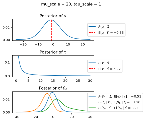
In this way, a large { \dot\sigma_{\mu} } and small { \dot\sigma_{\tau} } would create a model that assumes departments are relatively homogeneous (due to small \tau) but is very flexible about where the overall population mean might be (due to large \mu scale). This combination would result in strong shrinkage of department-specific estimates toward a population mean that is itself quite adaptable to the data. Conversely, a small { \dot\sigma_{\mu} } and large { \dot\sigma_{\tau} } would create a model that strongly believes the population mean is near zero, but allows substantial variation between departments.

param_list = [
    dict(mu_scale=1, tau_scale=1),
    # dict(mu_scale=5, tau_scale=5),
    # dict(mu_scale=10, tau_scale=10),
    dict(mu_scale=20, tau_scale=20),
    # dict(mu_scale=10, tau_scale=1),
    dict(mu_scale=20, tau_scale=3),
    # dict(mu_scale=1, tau_scale=10),
    dict(mu_scale=3, tau_scale=20),
]
for i_params_, params_ in enumerate(param_list):
    plot_model(**params_, figsize=(6, 5), verbose=True)

mu_scale=1, tau_scale=1 : E[θG | t]=0.139, Var[θG | t]=17.512
mu_scale=1, tau_scale=1 : E[θE | t]=-1.247, Var[θE | t]=24.192
mu_scale=1, tau_scale=1 : E[θM | t]=3.798, Var[θM | t]=55.836

mu_scale=20, tau_scale=20 : E[θG | t]=2.517, Var[θG | t]=112.461
mu_scale=20, tau_scale=20 : E[θE | t]=-6.000, Var[θE | t]=129.325
mu_scale=20, tau_scale=20 : E[θM | t]=16.936, Var[θM | t]=112.901

mu_scale=20, tau_scale=3 : E[θG | t]=3.228, Var[θG | t]=74.198
mu_scale=20, tau_scale=3 : E[θE | t]=-2.422, Var[θE | t]=87.779
mu_scale=20, tau_scale=3 : E[θM | t]=13.039, Var[θM | t]=83.766

mu_scale=3, tau_scale=20 : E[θG | t]=0.632, Var[θG | t]=78.673
mu_scale=3, tau_scale=20 : E[θE | t]=-5.378, Var[θE | t]=96.102
mu_scale=3, tau_scale=20 : E[θM | t]=13.063, Var[θM | t]=124.248

…vvv Shrinkage represents what statisticians call statistical information transfer between groups. Information about the Mathematics department indirectly influences our beliefs about the English department through their shared connection to the population-level parameters.

This statistical information transfer parallels a fundamental aspect of human cognition called inductive generalization—the ability to apply knowledge from one domain to another based on their perceived similarities or shared membership in a more abstract category. Just as observing many Golden Retrievers helps us form expectations about Dalmatians (through the shared category “dog”), observing Mathematics professors helps us form expectations about English professors (through the shared category “professor”).

The Role of Higher-Order Priors in Hierarchical Inference

The higher-order distributions we place on μ and τ (controlled by mu_scale and tau_scale) significantly influence the model’s inductive biases. These priors represent meta-level beliefs about the structure of department-specific patterns.

When mu_scale (σ_μ) is small (e.g., 1), the model strongly expects professors university-wide to be punctual. When mu_scale is large (e.g., 20), the model remains open to the possibility that professors university-wide systematically arrive early or late.

Similarly, when tau_scale (σ_τ) is small (e.g., 1), the model expects departments to behave similarly to each other. When tau_scale is large (e.g., 20), the model accommodates the possibility that departments differ substantially in their typical arrival times.

These different prior settings correspond to different “overhypotheses” in cognitive terms—abstract beliefs about the patterns that govern lower-level categories. For instance, a small τ-scale corresponds to the overhypothesis “departments are similar in their punctuality behavior,” while a large τ-scale corresponds to “departments likely have distinctive punctuality norms.”

The Statistical Leverage of Abstraction

In statistical learning theory, the curse of dimensionality refers to how increasing the number of parameters in a model typically makes learning exponentially more difficult. As parameter count increases, we require exponentially more data to estimate them reliably, and computational demands grow dramatically.

Given this principle, one might expect that our hierarchical model—which has more parameters than either the complete pooling or no pooling models—would require more data for effective learning. Yet counterintuitively, hierarchical models often learn more efficiently from limited data.

Let’s examine how inference proceeds at different levels of our model as we accumulate more observations. First, we’ll create a more extensive simulated dataset with departments that exhibit different punctuality patterns:

# Simulated data - multiple professors per department
t_extended = jnp.array([
    [-5, 0, 5, 2, -3],  # Government professors (mean close to 0)
    [-12, -18, -15, -10, -20],  # English professors (mean around -15)
    [25, 35, 28, 30, 32],  # Math professors (mean around +30)
])

By tracking how quickly the model learns at different levels as we observe more data, we discover a striking pattern: the model often infers the population-level parameter μ more rapidly than it infers the department-specific parameters θ_d. With just a few observations across departments, the model forms reasonably accurate beliefs about professors in general, even while maintaining considerable uncertainty about specific departments.

This phenomenon, which we’ll call the statistical leverage of abstraction, stands in contrast to the curse of dimensionality. By structuring inference hierarchically, we can sometimes achieve more efficient statistical learning at higher levels of abstraction, even though these levels are more removed from direct observation.

This statistical leverage depends crucially on the structure of the observed data. When departments genuinely share some common patterns (i.e., when the hierarchical structure of the model aligns with the generative process that produced the data), the model can leverage these patterns for more efficient learning. If departments were completely unrelated in their behavior, this advantage would disappear.

This statistical advantage of hierarchical inference parallels an important feature of human cognition—our capacity to form useful abstractions from limited evidence. Children can form remarkably accurate generalizations about biological categories from just a few examples, suggesting they efficiently learn at multiple levels of abstraction simultaneously. …^^^

Multiple observations with missing data

What if the president instead had a large meeting with 7 professors and the departments were not equally represented? How would she update her beliefs given unequal observations? Let’s say that she invited 3 professors from the Department of Government, 3 from the Department of English, and 1 from the Department of Math. We can explore how modulating the higher-level hyperpriors changes her posterior inference about each department.

\begin{align*} \mu ~\sim&~ \mathcal{N}(0, \dot\sigma_{\mu}) \\ \tau ~\sim&~ \text{HalfCauchy}(\dot\sigma_{\tau}) \\ \theta_d ~\sim&~ \mathcal{N}\left(\mu, \tau \right) \\ t_{(d,i)} ~\sim&~ \mathcal{N}(\theta_d, \dot\sigma{=}15) \\ d ~\in&~ D,~~~ \text{where}~~~ D = \{\text{G}, \text{E}, \text{M} \} \end{align*}

This extension demonstrates how multilevel models elegantly handle unbalanced data. Departments with more observations (Government and English) will have posterior distributions more heavily influenced by their own empirical data. The Math department, with just one observation, will have its posterior more strongly influenced by the population-level information - a phenomenon known as partial pooling or shrinkage.

The degree of shrinkage for each department depends on both the amount of department-specific data and the estimated between-department variance (τ). When τ is small (suggesting departments are similar), shrinkage will be stronger, especially for departments with limited data. When τ is large (suggesting substantial differences between departments), each department’s estimate will stay closer to its own empirical mean.

This behavior illustrates a fundamental advantage of multilevel models: they automatically adjust the degree of pooling based on the data, borrowing strength across groups in a principled way while preserving important group-level differences.

%reset -f
import jax
import jax.numpy as jnp
from memo import memo
from enum import IntEnum
from jax.scipy.stats.norm import pdf as normpdf
from jax.scipy.stats.norm import logpdf as normlogpdf
from jax.scipy.stats.cauchy import pdf as cauchypdf
from matplotlib import pyplot as plt

normpdfjit = jax.jit(normpdf)

class Department(IntEnum):
    GOVERNMENT = 0
    ENGLISH = 1
    MATH = 2

###NEW
t = jnp.array([
    [-10, 1, 11], 
    [-16, -15, -14], 
    [30, jnp.nan, jnp.nan],
])

sigma = 15

Mu = jnp.linspace(-25, 25, 100)
Tau = jnp.linspace(1, 30, 100)
Theta = jnp.linspace(-40, 40, 200)

@jax.jit
def half_cauchy(x, scale=1.0):
    return 2 * cauchypdf(x, 0, scale)

@jax.jit
def professor_arrival_likelihood(d, theta):
    ### likelihood of a professor from department d 
    ### showing up t_d minutes early/late, 
    ### for a given theta and sigma.
    return jnp.exp(jnp.nansum(normlogpdf(t[d], theta, sigma)))  ###NEW

@memo
def department_model[_mu: Mu, _tau: Tau](d):
    department: knows(_mu, _tau)
    department: chooses(theta in Theta, wpp=normpdfjit(theta, _mu, _tau))
    return E[ department[professor_arrival_likelihood(d, theta)] ]

@memo
def partial_pooling[_mu: Mu, _tau: Tau](mu_scale=5, tau_scale=5):
    president: knows(_mu, _tau)
    president: thinks[
        population: chooses(mu in Mu, wpp=normpdfjit(mu, 0, mu_scale)),
        population: chooses(tau in Tau, wpp=half_cauchy(tau, tau_scale)),
    ]
    president: observes_event(wpp=department_model[population.mu, population.tau]({Department.GOVERNMENT}))
    president: observes_event(wpp=department_model[population.mu, population.tau]({Department.ENGLISH}))
    president: observes_event(wpp=department_model[population.mu, population.tau]({Department.MATH}))
    return president[Pr[population.mu == _mu, population.tau == _tau]]

@memo
def department_model_theta[_theta: Theta](d, mu_scale, tau_scale):
    obs: thinks[
        department: chooses(mu in Mu, tau in Tau, wpp=partial_pooling[mu, tau](mu_scale, tau_scale)),
        department: chooses(theta in Theta, wpp=normpdfjit(theta, mu, tau))
    ]
    obs: observes_event(wpp=professor_arrival_likelihood(d, department.theta))
    obs: knows(_theta)
    return obs[Pr[department.theta == _theta]]

def plot_model(mu_scale=1, tau_scale=1, figsize=(10, 8)):
    posterior = partial_pooling(mu_scale=mu_scale, tau_scale=tau_scale)

    # Marginal over Tau (sum over Mu)
    posterior_tau = posterior.sum(axis=0)
    # Marginal over Mu (sum over Tau)
    posterior_mu = posterior.sum(axis=1)

    fig, axs = plt.subplots(3, 1, figsize=figsize)

    ax = axs[0]
    ax.axvline(0, color="black", linestyle="-")
    ax.plot(Mu, posterior_mu, label=r"$P(\mu \mid t)$")
    mu_expectation = jnp.dot(Mu, posterior_mu)
    ax.axvline(
        mu_expectation, 
        color='red', 
        linestyle='--', 
        label=r"$\operatorname{E}" + rf"[\mu \mid t]={mu_expectation:0.2f}$")
    _ = ax.set_title(r"Posterior of $\mu$")
    _ = ax.legend(bbox_to_anchor=(0.9, 0.5), loc='center left')

    ax = axs[1]
    ax.axvline(0, color="black", linestyle="-")
    ax.plot(Tau, posterior_tau, label=r"$P(\tau \mid t)$")
    tau_expectation = jnp.dot(Tau, posterior_tau)
    ax.axvline(
        tau_expectation, 
        color='red', 
        linestyle='--', 
        label=r"$\operatorname{E}" + rf"[\tau \mid t]={tau_expectation:0.2f}$")
    _ = ax.set_title(r"Posterior of $\tau$")
    _ = ax.legend(bbox_to_anchor=(0.9, 0.5), loc='center left')

    ax = axs[2]
    ax.axvline(0, color="black", linestyle="-")
    for d in Department:
        department_name = d.name
        department_abbrev = department_name[0]
        theta_posterior = department_model_theta(d, mu_scale, tau_scale)
        theta_expectation = jnp.dot(Theta, theta_posterior)
        ax.plot(
            Theta, 
            theta_posterior, 
            label=(
                rf"$P(\theta_{department_abbrev} \mid t),~ " 
                + r"\operatorname{E}" 
                + rf"[\theta_{department_abbrev} \mid t]={theta_expectation:0.2f}$"))
    _ = ax.set_title(r"Posterior of $\theta_d$")
    _ = ax.legend(bbox_to_anchor=(0.9, 0.5), loc='center left')

    _ = plt.suptitle(f"mu_scale = {mu_scale}, tau_scale = {tau_scale}", y=1)
    plt.tight_layout()
    plt.show()

param_list = [
    dict(mu_scale=1, tau_scale=1),
    # dict(mu_scale=5, tau_scale=5),
    # dict(mu_scale=10, tau_scale=10),
    dict(mu_scale=20, tau_scale=20),
    # dict(mu_scale=10, tau_scale=1),
    dict(mu_scale=20, tau_scale=1),
    # dict(mu_scale=1, tau_scale=10),
    dict(mu_scale=1, tau_scale=20),
]
for i_params_, params_ in enumerate(param_list):
    plot_model(**params_, figsize=(6, 5))

… (please finish)

Multiple observations with missing data and learned variance

Extended Model: Department-Specific Variability

Thus far, we’ve assumed uniform within-department variability (fixed at σ=15). However, departments might differ not only in their central tendencies but also in their internal consistency.

Let’s extend our model to infer department-specific variability:

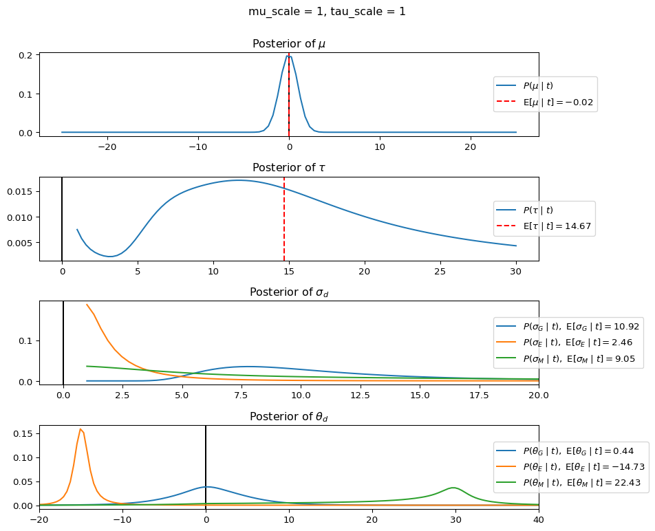
In our final model extension, we allow each department to have its own variance parameter \sigma_d, rather than fixing it at 15 for all departments:

Partial Variance Pooling with learned \sigma_d

\begin{align*} \mu ~\sim&~ \mathcal{N}(0, \dot\sigma_{\mu}) \\ \tau ~\sim&~ \text{HalfCauchy}(\dot\sigma_{\tau}) \\ \theta_d ~\sim&~ \mathcal{N}(\mu, \tau) \\ \sigma_d ~\sim&~ \text{HalfCauchy}(5) \\ t_{(d,i)} ~\sim&~ \mathcal{N}(\theta_d, \sigma_d) \\ d ~\in&~ \{ 0, 1, 2\} \end{align*}

This extension adds another hierarchical component by learning department-specific variance parameters \sigma_d. This allows the model to capture not just differences in mean arrival times between departments, but also differences in the consistency of professors within each department.

Departments where professors show similar punctuality behavior will have smaller \sigma_d values, while departments with more variable timing will have larger \sigma_d values. In our example, we might find that the English department has a small \sigma_E, indicating consistent punctuality behavior, while the Math department might have a larger \sigma_M, reflecting more variable arrival times.

This additional flexibility provides several benefits:

1. Improved model fit: By allowing department-specific variances, we can better capture the true data-generating process if departments genuinely differ in their consistency.

2. Heteroskedasticity handling: The model now properly accounts for differing levels of noise across departments.

3. Inference protection: Departments with highly consistent behavior won’t be overly influenced by more variable departments, as the model recognizes the difference in reliability.

4. Richer insights: Beyond just learning about average arrival times, we now learn about the predictability of professors from each department.

---

This extended model infers not just the typical arrival time for each department (θ_d) but also how consistent professors within that department are (σ_d). This allows the model to capture richer patterns, such as “English professors are consistently early” versus “Mathematics professors are late but with high variability.”

This additional modeling flexibility parallels how humans learn category structure. We learn not just the central tendencies of categories but also which features are consistent within a category and which are variable. For instance, we learn that mammals consistently have fur and give birth to live young (low variability features) but vary considerably in size and coloration (high variability features).

Learning Prototypes Across Departments

Our hierarchical model naturally corresponds to prototype learning in cognitive science. The population distribution parameterized by μ and τ captures the “prototype” of professor punctuality in general, while the department-specific parameters θ_d represent department-specific variations on this general prototype.

To make this correspondence explicit, let’s formulate a version of our model that directly represents the population-level prototype:

%reset -f
import jax
import jax.numpy as jnp
from memo import memo
from enum import IntEnum
from jax.scipy.stats.norm import pdf as normpdf
from jax.scipy.stats.norm import logpdf as normlogpdf
from jax.scipy.stats.cauchy import pdf as cauchypdf
from matplotlib import pyplot as plt

normpdfjit = jax.jit(normpdf)

class Department(IntEnum):
    GOVERNMENT = 0
    ENGLISH = 1
    MATH = 2

t = jnp.array([
    [-10, 1, 11], 
    [-16, -15, -14], 
    [30, jnp.nan, jnp.nan],
])

Mu = jnp.linspace(-25, 25, 100)
Tau = jnp.linspace(1, 30, 100)
Theta = jnp.linspace(-40, 40, 200)
Sigma = jnp.linspace(1, 30, 100)  ###NEW

@jax.jit
def half_cauchy(x, scale=1.0):
    return 2 * cauchypdf(x, 0, scale)

@jax.jit
def professor_arrival_likelihood(d, theta, sigma): ###NEW
    ### likelihood of a professor from department d 
    ### showing up t_d minutes early/late, 
    ### for a given theta and sigma.
    return jnp.exp(jnp.nansum(normlogpdf(t[d], theta, sigma)))

@memo(cache=True)
def department_model[_mu: Mu, _tau: Tau](d):
    department: knows(_mu, _tau)
    department: chooses(theta in Theta, wpp=normpdfjit(theta, _mu, _tau))
    department: chooses(sigma in Sigma, wpp=half_cauchy(sigma, 5))  ###NEW
    return E[ department[professor_arrival_likelihood(d, theta, sigma)] ]  ###NEW

@memo(cache=True)
def partial_pooling[_mu: Mu, _tau: Tau](mu_scale=5, tau_scale=5):
    president: knows(_mu, _tau)
    president: thinks[
        population: chooses(mu in Mu, wpp=normpdfjit(mu, 0, mu_scale)),
        population: chooses(tau in Tau, wpp=half_cauchy(tau, tau_scale)),
    ]
    president: observes_event(wpp=department_model[population.mu, population.tau]({Department.GOVERNMENT}))
    president: observes_event(wpp=department_model[population.mu, population.tau]({Department.ENGLISH}))
    president: observes_event(wpp=department_model[population.mu, population.tau]({Department.MATH}))
    return president[Pr[population.mu == _mu, population.tau == _tau]]

@memo(cache=True)
def department_model_theta[_theta: Theta](d, mu_scale, tau_scale):
    obs: thinks[
        department: chooses(mu in Mu, tau in Tau, wpp=partial_pooling[mu, tau](mu_scale, tau_scale)),
        department: chooses(theta in Theta, wpp=normpdfjit(theta, mu, tau)),
        department: chooses(sigma in Sigma, wpp=half_cauchy(sigma, 5)),  ###NEW
    ]
    obs: observes_event(wpp=professor_arrival_likelihood(d, department.theta, department.sigma))  ###NEW
    obs: knows(_theta)
    return obs[Pr[department.theta == _theta]]

@memo(cache=True)
def department_model_sigma[_sigma: Sigma](d, mu_scale, tau_scale):  ###NEW
    obs: thinks[
        department: chooses(mu in Mu, tau in Tau, wpp=partial_pooling[mu, tau](mu_scale, tau_scale)),
        department: chooses(theta in Theta, wpp=normpdfjit(theta, mu, tau)),
        department: chooses(sigma in Sigma, wpp=half_cauchy(sigma, 5)),
    ]
    obs: observes_event(wpp=professor_arrival_likelihood(d, department.theta, department.sigma))
    obs: knows(_sigma)
    return obs[Pr[department.sigma == _sigma]]

# Cache for precomputed results
cache = {}

def compute_distributions(mu_scale, tau_scale, verbose=False):
    """Retrieve from cache or compute the JAX-based distributions."""
    key = (mu_scale, tau_scale)
    if key in cache:
        return cache[key]  # Use cached results

    if verbose:
        print(f"{mu_scale=}, {tau_scale=}")

    # Cache results
    cache[key] = (
        partial_pooling(mu_scale=mu_scale, tau_scale=tau_scale).sum(axis=1), 
        partial_pooling(mu_scale=mu_scale, tau_scale=tau_scale).sum(axis=0), 
        {d: department_model_sigma(d, mu_scale, tau_scale) for d in Department}, 
        {d: department_model_theta(d, mu_scale, tau_scale) for d in Department},
    )
    return cache[key]

def plot_model(mu_scale=1, tau_scale=1, figsize=(10, 8)):
    posterior_mu, posterior_tau, sigma_posteriors, theta_posteriors = compute_distributions(mu_scale, tau_scale)

    fig, axs = plt.subplots(4, 1, figsize=figsize)

    ax = axs[0]
    ax.axvline(0, color="black", linestyle="-")
    ax.plot(Mu, posterior_mu, label=r"$P(\mu \mid t)$")
    mu_expectation = jnp.dot(Mu, posterior_mu)
    ax.axvline(
        mu_expectation, 
        color='red', 
        linestyle='--', 
        label=r"$\operatorname{E}" + rf"[\mu \mid t]={mu_expectation:0.2f}$")
    _ = ax.set_title(r"Posterior of $\mu$")
    _ = ax.legend(bbox_to_anchor=(0.9, 0.5), loc='center left')

    ax = axs[1]
    ax.axvline(0, color="black", linestyle="-")
    ax.plot(Tau, posterior_tau, label=r"$P(\tau \mid t)$")
    tau_expectation = jnp.dot(Tau, posterior_tau)
    ax.axvline(
        tau_expectation, 
        color='red', 
        linestyle='--', 
        label=r"$\operatorname{E}" + rf"[\tau \mid t]={tau_expectation:0.2f}$")
    _ = ax.set_title(r"Posterior of $\tau$")
    _ = ax.legend(bbox_to_anchor=(0.9, 0.5), loc='center left')

    ax = axs[2]
    ax.axvline(0, color="black", linestyle="-")
    for d in Department:
        department_name = d.name
        department_abbrev = department_name[0]
        sigma_posterior = sigma_posteriors[d]
        sigma_expectation = jnp.dot(Sigma, sigma_posterior)
        ax.plot(
            Sigma, 
            sigma_posterior, 
            label=(
                rf"$P(\sigma_{department_abbrev} \mid t),~ " 
                + r"\operatorname{E}" 
                + rf"[\sigma_{department_abbrev} \mid t]={sigma_expectation:0.2f}$"))
    _ = ax.set_xlim(-1, 20)
    _ = ax.set_title(r"Posterior of $\sigma_d$")
    _ = ax.legend(bbox_to_anchor=(0.9, 0.5), loc='center left')

    ax = axs[3]
    ax.axvline(0, color="black", linestyle="-")
    for d in Department:
        department_name = d.name
        department_abbrev = department_name[0]
        theta_posterior = theta_posteriors[d]
        theta_expectation = jnp.dot(Theta, theta_posterior)
        ax.plot(
            Theta, 
            theta_posterior, 
            label=(
                rf"$P(\theta_{department_abbrev} \mid t),~ " 
                + r"\operatorname{E}" 
                + rf"[\theta_{department_abbrev} \mid t]={theta_expectation:0.2f}$"))
    _ = ax.set_xlim(-20, 40)
    _ = ax.set_title(r"Posterior of $\theta_d$")
    _ = ax.legend(bbox_to_anchor=(0.9, 0.5), loc='center left')

    _ = plt.suptitle(f"mu_scale = {mu_scale}, tau_scale = {tau_scale}", y=1)
    plt.tight_layout()
    plt.show()

param_list = [
    dict(mu_scale=1, tau_scale=1),
    # dict(mu_scale=5, tau_scale=5),
    dict(mu_scale=10, tau_scale=10),
    # dict(mu_scale=20, tau_scale=20),
    dict(mu_scale=10, tau_scale=1),
    # dict(mu_scale=20, tau_scale=1),
    dict(mu_scale=1, tau_scale=10),
    # dict(mu_scale=1, tau_scale=20),
]
plt.close("all")
for i_params_, params_ in enumerate(param_list):
    plot_model(**params_, figsize=(10, 8))

The plot shows how different combinations of hyperparameters (\dot\sigma_{\mu} and \dot\sigma_{\tau}) affect the posterior distributions of \mu, \tau, \sigma_d, and \theta_d. By examining these interactions, we can gain deeper insights into how multilevel models balance population-level information with group-specific data.

---

Exercises

1. Model Comparison: Implement the complete pooling, no pooling, and partial pooling models for a new dataset. Calculate the posterior predictive distributions for each model and compare their predictive performance using measures like mean squared error or log likelihood.

2. Hyperparameter Sensitivity: Investigate how sensitive the partial pooling model’s inferences are to different values of \dot\sigma_{\mu} and \dot\sigma_{\tau}. Create a grid of values and visualize how the posterior means and variances of \theta_d change across this grid.

3. New Department Prediction: Extend the model to predict the arrival time of a professor from a new, previously unobserved department (e.g., Psychology). Compare predictions from all three modeling approaches and discuss which makes the most reasonable predictions.

4. Skewed Distributions: Modify the model to use a skewed distribution (e.g., log-normal or skew-normal) for arrival times, since lateness might follow a different pattern than earliness. How does this change the inferences?

5. Covariate Extension: Extend the partial pooling model to include a covariate such as years of teaching experience or time of day. The model could be: \theta_d = \mu + \beta x_d + \eta_d, \text{ where } \eta_d \sim \mathcal{N}(0, \tau) Implement this model and discuss how it changes your inferences.

These exercises will deepen your understanding of multilevel models and their application to real-world hierarchical data structures.

Further reading

• McElreath (2016, Chapters 1, 13, 14)
• Gelman (2014, Chapter 5)
• Kruschke (2015, Chapter 9)

---

@memo
def prototype_learning[_arrival_time: ArrivalTimes]:
    president: thinks[
        population: chooses(mu in Mu, wpp=normpdfjit(mu, 0, 10)),
        population: chooses(tau in Tau, wpp=half_cauchy(tau, 10)),
        population: chooses(prototype_time in ArrivalTimes, 
                            wpp=normpdfjit(prototype_time, population.mu, population.tau))
    ]
    
    # Observe data from multiple departments
    president: observes_event(
        wpp=department_data_likelihood(Department.GOVERNMENT, population.mu, population.tau))
    president: observes_event(
        wpp=department_data_likelihood(Department.ENGLISH, population.mu, population.tau))
    president: observes_event(
        wpp=department_data_likelihood(Department.MATH, population.mu, population.tau))
    
    president: knows(_arrival_time)
    return president[Pr[population.prototype_time == _arrival_time]]

This model explicitly queries the prototype arrival time for professors in general. From observations across multiple departments, the model infers a prototype that balances commonalities across departments (influenced by μ) while accounting for department-specific variations (influenced by τ).

This process parallels how humans might form the prototype for a basic-level category like “dog” from experiences with different subordinate categories (breeds). The prototype captures central tendencies across breeds while abstracting away breed-specific variations.

Learning Overhypotheses About Departmental Structure

Let’s examine how our model learns overhypotheses—abstract knowledge about the structure of punctuality patterns across departments. One crucial overhypothesis concerns the question: “How similar are departments to each other in their punctuality behavior?”

We can capture this by focusing on the posterior distribution of τ:

@memo
def overhypothesis_learning[_tau: Tau](data, tau_scale=10):
    president: knows(_tau)
    president: thinks[
        population: chooses(mu in Mu, wpp=normpdfjit(mu, 0, 10)),
        population: chooses(tau in Tau, wpp=half_cauchy(tau, tau_scale))
    ]
    
    # Observe data
    for dept in Department:
        for i in range(len(data[dept])):
            if not jnp.isnan(data[dept][i]):
                president: observes_event(
                    wpp=professor_arrival_likelihood_for_overhypothesis(dept, i, 
                                                                        population.mu, population.tau))
    
    return president[Pr[population.tau == _tau]]

Let’s consider two contrasting datasets:

# Scenario 1: Departments exhibit similar arrival patterns
similar_departments_data = jnp.array([
    [5, 6, 4, 5, 6],  # Government (around +5)
    [4, 7, 5, 6, 4],  # English (around +5) 
    [6, 5, 4, 6, 5],  # Math (around +5)
])

# Scenario 2: Departments exhibit distinct arrival patterns
different_departments_data = jnp.array([
    [0, 2, -1, 1, 0],     # Government (around 0)
    [-15, -16, -14, -15, -16],  # English (around -15)
    [30, 28, 31, 30, 29],  # Math (around +30)
])

When we run our overhypothesis_learning model on these datasets, we find that τ tends to be small for the similar_departments_data and large for the different_departments_data. This represents learning the overhypothesis “departments have similar punctuality patterns” versus “departments have distinctive punctuality norms.”

This overhypothesis learning parallels how humans learn abstract principles like “animals of the same species have the same number of legs” or “members of the same tribe typically share physical characteristics.” These abstract principles guide efficient inference when we encounter new examples, allowing us to make strong predictions from limited evidence.

One-Shot Learning Through Hierarchical Structure

One of the most remarkable capacities enabled by hierarchical mental representations is one-shot learning—the ability to make strong inferences from a single observation. Let’s examine how our model handles one-shot learning for a previously unobserved department:

@memo
def one_shot_learning[_arrival_time: ArrivalTimes](observed_time):
    president: thinks[
        population: chooses(mu in Mu, wpp=normpdfjit(mu, 0, 10)),
        population: chooses(tau in Tau, wpp=half_cauchy(tau, 10)),
        
        # Existing departments
        govt_dept: chooses(theta in Theta, wpp=normpdfjit(theta, population.mu, population.tau)),
        english_dept: chooses(theta in Theta, wpp=normpdfjit(theta, population.mu, population.tau)),
        math_dept: chooses(theta in Theta, wpp=normpdfjit(theta, population.mu, population.tau)),
        
        # New department (Psychology)
        psych_dept: chooses(theta in Theta, wpp=normpdfjit(theta, population.mu, population.tau)),
        
        # First observation of Psychology professor
        psych_first_obs: chooses(time in ArrivalTimes, 
                                 wpp=normpdfjit(time, psych_dept.theta, 15)),
        
        # Future observation of Psychology professor
        psych_future_obs: chooses(time in ArrivalTimes, 
                                 wpp=normpdfjit(time, psych_dept.theta, 15))
    ]
    
    # Observe existing department data
    president: observes_event(
        wpp=department_data_likelihood(Department.GOVERNMENT, population.mu, population.tau))
    president: observes_event(
        wpp=department_data_likelihood(Department.ENGLISH, population.mu, population.tau))
    president: observes_event(
        wpp=department_data_likelihood(Department.MATH, population.mu, population.tau))
    
    # Observe first Psychology professor
    president: observes [psych_first_obs.time] is observed_time
    
    # Query future Psychology professor's arrival time
    president: knows(_arrival_time)
    return president[Pr[psych_future_obs.time == _arrival_time]]

This model captures one-shot learning for a new department (Psychology). After observing just one Psychology professor with a particular arrival time, the model forms expectations about future Psychology professors.

The strength of these expectations depends crucially on the learned overhypothesis about departmental similarity (τ). If τ is small (departments are similar), the single observation will have limited influence, and predictions will be heavily influenced by the population mean. If τ is large (departments differ substantially), the single observation will strongly shape predictions about future Psychology professors.

This one-shot learning capacity parallels how humans make strong inferences from limited evidence. Upon seeing a new animal species with eight legs, we confidently predict that other members of the same species will also have eight legs—a prediction guided by our overhypothesis that leg count is consistent within species.

Applying Hierarchical Models to Concept Learning: The Shape Bias

Our departmental punctuality models have direct parallels to concept learning in cognitive development. Consider the well-documented “shape bias” in children’s word learning—the tendency to generalize object names based on shape rather than color or texture.

We can reinterpret our model in terms of object properties:

@memo
def shape_bias_model[_feature_type: FeatureType, _value: FeatureValue](
    new_object_category, feature_type, observed_value):
    
    learner: thinks[
        # Different concentration parameters for different feature dimensions
        shape_alpha: chooses(alpha in Alpha, wpp=exponential_pdf(alpha, 1)),
        color_alpha: chooses(alpha in Alpha, wpp=exponential_pdf(alpha, 1)),
        texture_alpha: chooses(alpha in Alpha, wpp=exponential_pdf(alpha, 1)),
        
        # Global prototypes for each feature dimension
        shape_prototype: chooses(proto in FeaturePrototype, 
                                wpp=dirichlet_pdf(proto, ones(shape_values))),
        color_prototype: chooses(proto in FeaturePrototype, 
                                wpp=dirichlet_pdf(proto, ones(color_values))),
        texture_prototype: chooses(proto in FeaturePrototype, 
                                  wpp=dirichlet_pdf(proto, ones(texture_values))),
        
        # Category-specific feature distributions
        category: chooses(
            shape_dist in FeatureDistribution, 
            wpp=dirichlet_pdf(shape_dist, shape_alpha * shape_prototype)),
        category: chooses(
            color_dist in FeatureDistribution, 
            wpp=dirichlet_pdf(color_dist, color_alpha * color_prototype)),
        category: chooses(
            texture_dist in FeatureDistribution, 
            wpp=dirichlet_pdf(texture_dist, texture_alpha * texture_prototype)),
        
        # Sample feature values for the new object
        new_object: chooses(
            shape in FeatureValue, 
            color in FeatureValue,
            texture in FeatureValue,
            wpp=category.shape_dist[shape] * 
                category.color_dist[color] * 
                category.texture_dist[texture])
    ]
    
    # Observe training data (multiple object categories with consistent shapes)
    learner: observes_event(wpp=training_data_likelihood(...))
    
    # Observe single instance of new category
    learner: observes [new_object.feature_type] is observed_value
    
    # Query: how likely are different feature types and values for future objects in this category?
    learner: knows(_feature_type, _value)
    return learner[Pr[new_object.feature_type == _value]]

This model captures how children might learn the shape bias from observing that objects with the same name tend to have the same shape (low shape_alpha) but may vary in color or texture (higher color_alpha and texture_alpha). After learning these different concentration parameters, the model will show a bias to generalize new object names based on shape rather than other properties.

Just as our university president learned which aspects of professor punctuality are consistent within departments, children learn which object properties are consistent within named categories. This learning of different levels of feature variability represents a sophisticated form of overhypothesis acquisition that guides future learning.

The Statistical Leverage of Abstraction in Hierarchical Knowledge

Throughout this chapter, we’ve encountered a counterintuitive phenomenon: hierarchical structuring of representations often facilitates more efficient learning rather than complicating it. This “statistical leverage of abstraction” emerges because:

1. Higher-level abstractions can be efficiently inferred from diverse but limited data
2. These abstractions then constrain lower-level inferences, enabling strong predictions from sparse evidence
3. When the structure of representations aligns with the structure of the generative process that produced the data, inference becomes more statistically efficient

This stands in contrast to the “curse of dimensionality,” which suggests that adding parameters should make learning more statistically challenging. The key insight is that hierarchical organization doesn’t merely add parameters—it adds structure that, when appropriately aligned with the data-generating process, facilitates more efficient inference.

We observed this statistical leverage most clearly in the learning curves analysis: with just a few observations across departments, our model formed meaningful abstractions about professors in general, which then guided department-specific inferences. This parallels how children can learn abstract principles (like “animals of the same species share anatomical features”) from limited but diverse examples, which then guide future inferences.

Conclusion: Hierarchical Models and the Structure of Mental Representations

Multilevel models provide a formal framework for understanding how mental representations might be organized hierarchically across multiple levels of abstraction. From our exploration of professor punctuality, we’ve seen how these models capture several fundamental aspects of human cognition:

1. Prototype Learning: The formation of central tendencies that characterize categories at different levels of abstraction
2. Statistical Information Transfer: The propagation of information between related entities through shared higher-level structure
3. Overhypothesis Learning: The acquisition of abstract principles about the structure of lower-level categories
4. One-Shot Learning: The capacity to make strong inferences from minimal evidence
5. The Statistical Leverage of Abstraction: The counterintuitive phenomenon where reasoning at higher levels of abstraction can be more statistically efficient than focusing exclusively on specific instances

These cognitive capacities emerge naturally from the mathematics of hierarchical Bayesian inference. By structuring representations hierarchically, with higher levels constraining lower levels, these models achieve a remarkable balance between flexibility and constraint—adapting to the unique patterns of specific entities while leveraging the common patterns shared across entities.

This hierarchical organization provides a computational account of how human mental representations might be structured—from specific instances to subordinate categories to basic-level categories to superordinate categories. Each level captures different statistical regularities and supports different kinds of generalizations.

The next time you find yourself making a prediction based on limited evidence—whether anticipating a colleague’s arrival time, judging a restaurant based on a single meal, or inferring an animal’s properties from a brief observation—consider the hierarchical mental representations that enable such predictions. What higher-level abstractions guide your inference? What overhypotheses constrain your predictions? And how might your observations at different levels of abstraction interact to shape your understanding?

Exercises

1. Model Comparison: Implement the complete pooling, no pooling, and partial pooling models for a dataset of your choice. Calculate the posterior predictive distributions for each model and analyze how they balance bias and variance in their inferences.

2. The Statistical Leverage of Abstraction: Design a simulation study to demonstrate how inference can be more efficient at higher levels of abstraction than at lower levels. Create datasets with different degrees of between-group similarity and analyze how this affects learning rates.

3. One-Shot Learning: Extend the partial pooling model to predict the arrival time of a professor from a new, previously unobserved department (e.g., Psychology) based on a single observation. Compare this prediction to what complete pooling and no pooling models would predict.

4. Overhypothesis Learning: Design a model that learns different concentration parameters for different feature dimensions (like the shape bias model). Apply it to a novel dataset and analyze what overhypotheses the model learns.

5. Learning Curves Analysis: Implement a study of learning curves at different levels of abstraction. Compare how quickly the model learns population parameters versus group-specific parameters as the amount of data increases.

6. Information Transfer: Design an experiment where the model first learns from several “source” departments, then encounters a “target” department with limited data. Measure how the learned hierarchical structure facilitates information transfer to the new department.

7. Feature Variability: Extend the model to learn which features of professors (e.g., arrival time, meeting preparation, speaking duration) are consistent within departments and which vary. How does this learning of feature-specific variability influence predictions?

8. Human Experiment Design: Design a behavioral experiment to test whether human inferences show the patterns of hierarchical learning predicted by these models. What specific predictions could you test?

Further Reading

• Gelman, A., & Hill, J. (2006). Data Analysis Using Regression and Multilevel/Hierarchical Models. Cambridge University Press.
• McElreath, R. (2020). Statistical Rethinking (2nd ed.). CRC Press.
• Kruschke, J. K. (2015). Doing Bayesian Data Analysis (2nd ed.). Academic Press.
• Kemp, C., Perfors, A., & Tenenbaum, J. B. (2007). Learning overhypotheses with hierarchical Bayesian models. Developmental Science, 10(3), 307-321.
• Tenenbaum, J. B., Kemp, C., Griffiths, T. L., & Goodman, N. D. (2011). How to grow a mind: Statistics, structure, and abstraction. Science, 331(6022), 1279-1285.

References

Gelman, Andrew. (2014). Bayesian data analysis (Third edition). CRC Press.

Kruschke, John K. (2015). Doing Bayesian data analysis: A tutorial with R, JAGS, and Stan (Edition 2). Academic Press.

McElreath, Richard. (2016). Statistical rethinking: A Bayesian course with examples in R and Stan. CRC Press/Taylor & Francis Group.