Demo: marimo Integration

Testing marimo notebook export from Quarto

marimo Notebook

This demo tests the marimo notebook export workflow. The .qmd source renders to HTML via Quarto, and can also be converted to a marimo .py notebook for interactive use.

Setup

import marimo as mo
from memo import memo
import jax.numpy as np
import jax
from matplotlib import pyplot as plt

The Guessing Game Model

We model a “guess 2/3 of the average” game where players try to guess a number that will be closest to 2/3 of the average of all guesses.

N = np.arange(100 + 1)  # space of possible guesses (0 to 100)

Defining the Player Model

The @memo decorator lets us express recursive reasoning compactly. Each player reasons about what others might choose, then picks accordingly.

@memo
def player[n: N](level, beta):
    """
    A level-k player reasons about level-(k-1) players.
    - level 0: uniform random choice
    - level k: best responds to level k-1 players
    - beta: rationality parameter (higher = more rational)
    """
    reader: thinks[
        everyone_else: chooses(n in N, wpp=player[n](level - 1, beta) if level > 0 else 1)
    ]
    reader: chooses(n in N, wpp=exp(beta * -abs(n - (2/3) * E[everyone_else.n])))
    return Pr[reader.n == n]

Timing the Model

Let’s measure how fast memo-lang can compute a level-10 player’s distribution.

import timeit

# Warm up JIT compilation
_ = player(10, 1.0).block_until_ready()

# Time 100 runs
times = timeit.repeat(
    lambda: player(10, 1.0).block_until_ready(),
    number=100,
    repeat=10
)
avg_time_ms = (min(times) / 100) * 1000

print(f"Level-10 player computation: {avg_time_ms:.3f} ms per call")
print(f"(Best of 10 runs, 100 calls each)")

Level-10 player computation: 0.306 ms per call
(Best of 10 runs, 100 calls each)

Visualizing Player Distributions

Different levels of reasoning produce different prediction distributions.

fig, ax = plt.subplots(figsize=(10, 6))

for level in range(5):
    distribution = player(level, beta=1.0)
    ax.plot(N, distribution, label=f'Level {level} player', linewidth=2)

ax.set_xticks(N[::10])
ax.set_xlabel('Guess (n)')
ax.set_ylabel('Predicted probability of choosing n')
ax.set_title('Player Behavior by Reasoning Level')
ax.legend()
ax.grid(True, alpha=0.3)

plt.tight_layout()
plt.show()

Text(0.5, 0, 'Guess (n)')

Text(0, 0.5, 'Predicted probability of choosing n')

Text(0.5, 1.0, 'Player Behavior by Reasoning Level')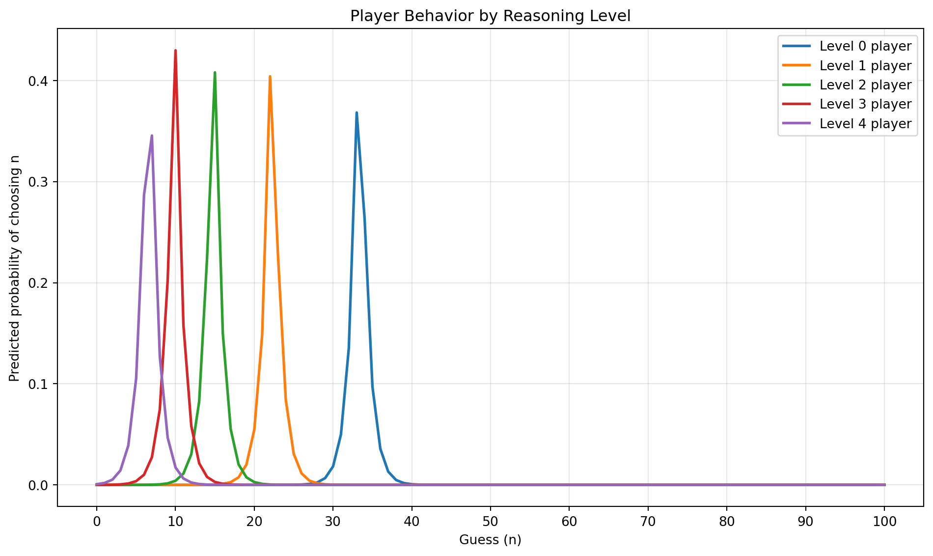

Interpretation

• Level 0: Uniform distribution (random guessing)
• Level 1: Best responds to random players, peaks near 33 (2/3 of 50)
• Level 2: Best responds to level-1 players, peaks near 22
• Higher levels: Distributions converge toward 0 (the Nash equilibrium)

The beta parameter controls how “rational” players are:

• Low beta: more random choices
• High beta: more deterministic best-response

Exploring Rationality

fig2, axes = plt.subplots(1, 3, figsize=(14, 4))

betas = [0.1, 1.0, 5.0]
for ax, beta in zip(axes, betas):
    for lvl in range(4):
        dist = player(lvl, beta=beta)
        ax.plot(N, dist, label=f'Level {lvl}')
    ax.set_title(f'beta = {beta}')
    ax.set_xlabel('Guess')
    ax.set_ylabel('Probability')
    ax.legend()
    ax.grid(True, alpha=0.3)

plt.suptitle('Effect of Rationality Parameter (beta) on Player Distributions')
plt.tight_layout()
plt.show()

Text(0.5, 1.0, 'beta = 0.1')

Text(0.5, 0, 'Guess')

Text(0, 0.5, 'Probability')

Text(0.5, 1.0, 'beta = 1.0')

Text(0.5, 0, 'Guess')

Text(0, 0.5, 'Probability')

Text(0.5, 1.0, 'beta = 5.0')

Text(0.5, 0, 'Guess')

Text(0, 0.5, 'Probability')

Text(0.5, 0.98, 'Effect of Rationality Parameter (beta) on Player Distributions')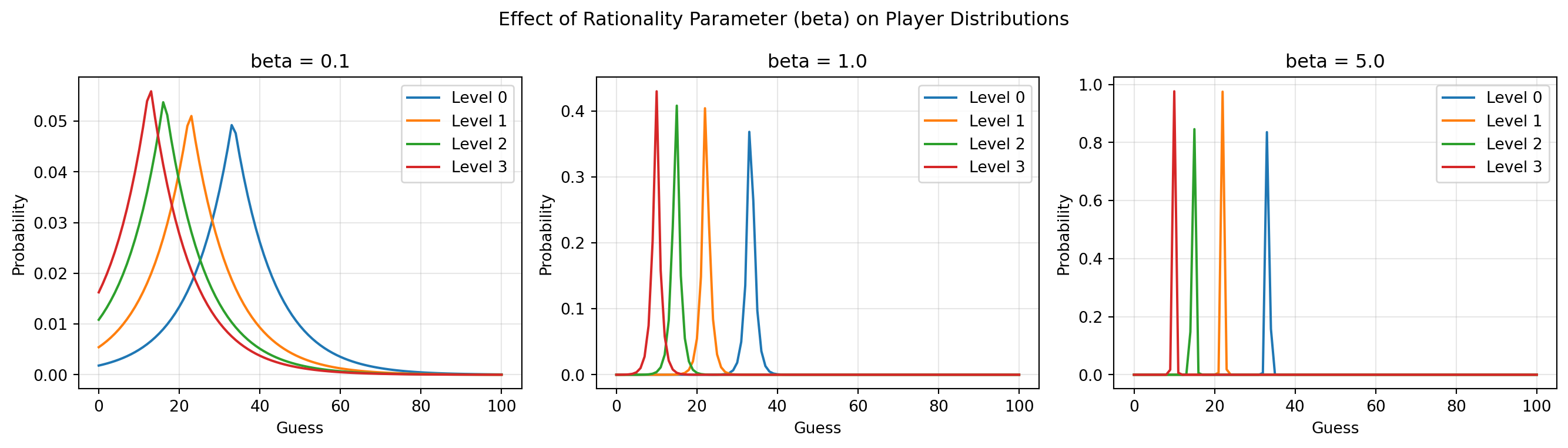

Running This Locally

To run this notebook interactively with full editing capabilities:

cd project
uv run marimo edit quartobook/notebooks_exported/demo-marimo.py